Exploring Word Vectors With GloVe and Gensim 🧭

An NLP primer on the computer representation of text

For machines to understand our language, we need to represent words numerically. We can do so with supervised or unsupervised ML techniques. After training our model, we can use the concept of similarity for various tasks, and in doing so, oh surprise, we run into bias! Read on to know more! (Jupyter Notebook included)

In late 2020 I began my exploration of AI. After the excellent introductory course at Columbia University and the Deep Learning lessons at MIT, it became clear to me that I want to pursue my career in this area.

I always liked and enjoyed mathematics, statistics, and other pure sciences while in college. Sadly I rarely used their concepts during my professional career as a CS Engineer. So, it was a pleasant surprise to see calculus, linear algebra, or probability distributions again during class!.

After some time exploring the applications of ML, I became very interested in NLP since other of my passions are knowledge, learning, and data/information management. That is why I decided to go back to the classroom. In this case, I choose Stanford's excellent CS224N (Natural Language Processing with Deep Learning) taught by the charismatic Professor Manning.

After the first assignment, I thought it would be interesting to record my impressions, experiences, and discoveries here for later reference or because it might be helpful to someone else.

Let's get down to business. In this article, I explore a fundamental concept of NLP: The representation of words so that machines can understand them.

Representing a word is not enough
- Count-Based Word Vectors
- Prediction-Based Word Vectors
Similarity
Playing around with GloVe and Gensim

Representing a word is not enough

It is easy to represent words as discrete symbols like hot-vectors. Unfortunately, such representations lack notions of similarity.

There are better solutions. The most common one represents words as dense vectors whose dimensions show degrees of similarity with other words that usually appear in their context.

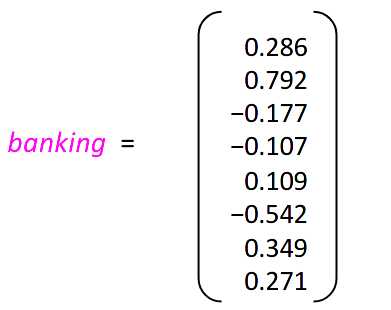
A word vector for banking (source: CS244N)

We can implement word vectors using count-based or prediction-based techniques.

Count-Based Word Vectors

In this technique, we use co-occurrence matrices to represent word embeddings. These symmetric matrices count the times a word happens in a context taking into account a fixed window $n$ surrounding a word $w_i$ .

These matrices are high dimensional given the nature of human language, so it is needed to apply dimensionality reduction techniques like SVD, PCA, or Truncated SVD to select the top $k$ components.

Prediction-Based Word Vectors

These approaches have better performance than count-based methods. There are two famous techniques to train the models. If we want an unsupervised method we can use Stanford's GloVe, otherwise, we can train a model with the word2vec framework.

word2vec comes in two flavors, both able to learn word embeddings: CBOW (Continuous bag-of-words) and SG (skip-gram). The skip-gram architecture is commonly used for its ability to predict rare words. Skip-gram tries to predict the $m$ words that are around a center word $w_t$ given a parameters vector $\theta$ which contains all word vectors in the corpus' vocabulary:

L(\theta) = \prod_{t=1}^{T} \prod_{-m \leq j \leq m} P(w_{t+j} | w_t; \theta); j \neq 0

The objective function, $J(\theta)$ , is the average negative $log$ of $L(\theta)$ which we want to minimize though SGD (notice that the vector space is enormous):

J(\theta) = - \frac{1}{T} \log L(\theta) = - \frac{1}{T} \sum_{t=1}^{T} \sum_{-m \leq j \leq m} \log P(w_{t+j} | w_t; \theta); j \neq 0

Similarity

Once we have trained our model, we can use it to make predictions based on the similarity concept. For this we can use a popular metric called $Cosine Similarity$ or better $Cosine Distance = (1 - CosineSimilarity)$ .

With this metric, we can find synonyms, antonyms, and even analogies among words.

Playing around with GloVe and Gensim

Once we have the word embeddings we can explore how well they have captured meaning. For this, we can use Gensim. Gensim is an excellent package to explore the similarity concept. Please check the related Jupyter Notebook to see how to do it in detail. In the next section, I present some highlights from the execution of the mentioned notebook.

Dependencies

numpy: For linear algebra tasks when working with matrices
matplotlib: To display word vectors in 2-D after dimensionality reduction
nltk: To work with the Reuter's corpus (10,788 news documents, 1.3 million words in 90 categories. The documents are split into train and test folders)
sklearn: To reduce the co-occurrence matrices dimensionality with PCA or Truncated SVD
gensim: To work with the pre-trained GloVe word embeddings

Count-Based Word Vectors

Creating the Co-Occurrence Matrix

To make things easier I created a function to determine the words in the vicinity of the center word $w_i$ :

  def _get_vicinity(w_i: str, corpus: list, window_size: int=4) -> list:
    """
    Returns a list with words located after or before of current word w_ij
    given a window_size. For example, if the corpus is
    [
      ['<START>', 'All', 'that', 'glitters', "isn't", 'gold', '<END>'],
      ['<START>', "All's", 'well', 'that', 'ends', 'well', '<END>']
    ]
    the vicinity/CONTEXT of "well" is: ["All's", 'that', 'ends', '<END>']

    Parameters
    ----------
    - w_i (str): The target word for which we'll determine its vicinity
    - corpus (list): A list of lists, each item represent a document
    - window_size (int): The range where we'll find neighbor words for w_i

    Returns
    -------
    A list of words which are neighbors of w_i given a window_size
    """
    
    neighbors = []

    for doc in corpus:
      if w_i in doc:  # The word can appear several time in the document!
        
        # Indices where w_i appears in the current document
        indices = [idx for idx, value in enumerate(doc) if value == w_i]

        for i in indices:
          lower_bound = i - window_size if i > window_size else 0
          upper_bound = i + 1 + window_size  # No error if x[i: out-of-bounds]

          neighbors.append(doc[lower_bound: i])
          neighbors.append(doc[i + 1: upper_bound])

    return [neighbor[0] for neighbor in neighbors if len(neighbor) > 0]

Dimensionality Reduction with Truncated SVD

This is an important note to take into account:

TruncatedSVD returns $U*S$ , then we need to normalize (rescale) the returned vectors so that all the vectors will appear around the unit circle. We achieve this normalization through the NumPy concept of broadcasting.

CS224N

Plot Analysys Between Count-Based and Prediction-Based Word Vectors

I used Gensim to load the glove-wiki-gigaword-200 and convert it to a word2vec representation. This model contains 400K words on its vocabulary! The results show a slightly better performance using the Prediction-Based approach (image on the right):

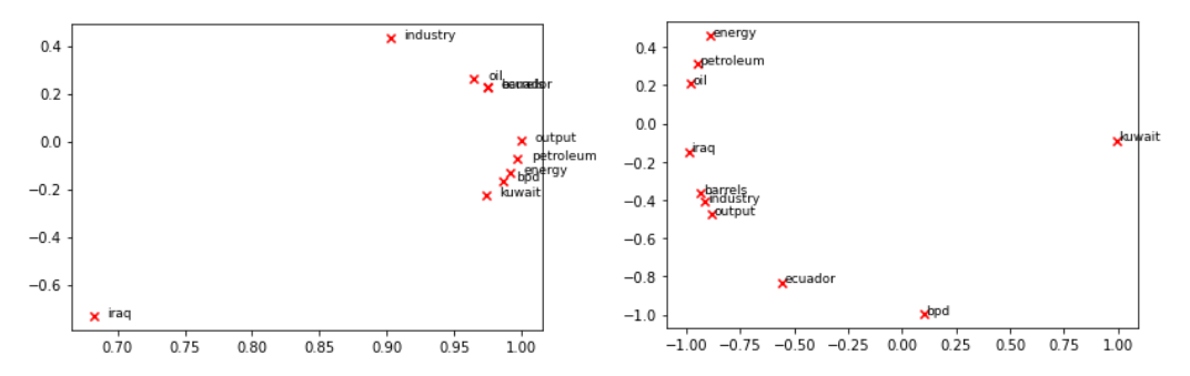
Count and prediction-based plots

In the Prediction-Based Model, we have a main cluster containing most of the words in the sample set. Nevertheless, it is still odd kuwait is far apart from words like oil. Why is this happening? Perhaps it is because we are using a small sample of 10K GloVe vectors, or it may also be related to the truncation done when reducing the dimensionality. Another possibility is that in the selected 10K GloVe vectors kuwait doesn't appear with enough frequency in the context of the other words.

Similarity: Polysemes, Synonyms, Antonyms, and Analogies

Gensim's method called most_similar allows us to perform the above tasks with ease. This method uses the concept of Cosine Similarity in its implementation. Some highlights about its usage:

most_similar without extra parameters returns the top 10 words most similar to the word passed as argument. Nevertheless, there are some polyseme cases not working as expected, for example for branch I couldn't find any tree/plant-related words:
```
wv_from_bin.most_similar("branch")

[('branches', 0.7101372480392456),
('central', 0.5476117730140686),
('railway', 0.5329204797744751),
('established', 0.5197478532791138),
('line', 0.5076225399971008),
('authority', 0.491929292678833),
('offices', 0.48285460472106934),
('railroad', 0.4816432297229767),
('headquarters', 0.4756273925304413),
('department', 0.4709719121456146)]
```
Why is that? It seems to me that it is related to the dataset used during the training process. It might happen that the dataset didn't have varied enough context for this word sense.
There are also some odd results when finding antonyms and synonyms. For instance, in the below example, the antonym is closer than the synonym:
```
# wv_from_bin.most_similar("top")

# w1 = top, w2 = pinnacle/summit/peak/apex, w3 = bottom
# w1 and w2 can be considered synonyms
# w1 and w3 can be considered antonyms

# Distance from synonyms are 0.76/0.67/0.67/0.79
# wv_from_bin.distance("top", "apex")

# Distance from antonym is 0.49
wv_from_bin.distance("top", "bottom")
```
Why is this happening? Here, I also guess it is because of the data used to train the model. Probably the training examples were rich in contexts for the word "top" that involved success, leadership, and businesses. But those contexts were not so rich in vocabulary.
We can use the most_similar method to find analogies. But here also, the results are not always satisfactory.
```
wv_from_bin.most_similar(positive=['hand', 'glove'], negative=['foot'])

45,000-square
```
I wonder if we'll get better results with a word2vec pre-trained model instead.

The Sad Reality of Bias

Word embeddings are susceptible to bias. This is dangerous because it can reinforce stereotypes through applications that employ these models.

CS224N

A classical example:

pprint.pprint(wv_from_bin.most_similar(positive=['woman', 'worker'], negative=['man']))
print()
pprint.pprint(wv_from_bin.most_similar(positive=['man', 'worker'], negative=['woman']))

[('employee', 0.6375863552093506),
('workers', 0.6068919897079468),
('nurse', 0.5837947726249695),
('pregnant', 0.5363885164260864),
('mother', 0.5321309566497803),
('employer', 0.5127025842666626),
('teacher', 0.5099576711654663),
('child', 0.5096741914749146),
('homemaker', 0.5019454956054688),
('nurses', 0.4970572590827942)]

[('workers', 0.6113258004188538),
('employee', 0.5983108282089233),
('working', 0.5615328550338745),
('laborer', 0.5442320108413696),
('unemployed', 0.5368517637252808),
('job', 0.5278826951980591),
('work', 0.5223963260650635),
('mechanic', 0.5088937282562256),
('worked', 0.505452036857605),
('factory', 0.4940453767776489)]

Since when nurse and teacher are "exclusive" jobs for women? Same for "mechanic".

Jennifer Beals welding, Flashdance, 1983

This is sad, and it is present in other examples:

pprint.pprint(wv_from_bin.most_similar(positive=['latin', 'criminal'], negative=['white']))
print()
pprint.pprint(wv_from_bin.most_similar(positive=['white', 'criminal'], negative=['latin']))

[('trafficking', 0.4996181130409241),
('transnational', 0.44992437958717346),
('crimes', 0.43998926877975464),
('laundering', 0.4213477373123169),
('crime', 0.42046865820884705),
('cartels', 0.417102575302124),
('dealing', 0.4154001474380493),
('traffickers', 0.40704718232154846),
('judicial', 0.39766523241996765),
('extradition', 0.3974517583847046)]

[('prosecution', 0.5594319105148315),
('crimes', 0.5117124915122986),
('fbi', 0.5068686008453369),
('attorney', 0.5007576942443848),
('investigation', 0.49686378240585327),
('charges', 0.49135079979896545),
('charged', 0.48554402589797974),
('prosecutors', 0.4846910238265991),
('attorneys', 0.47757965326309204),
('suit', 0.476983904838562)]

How can we avoid this? Not sure. The only thing I can think of is taking random samples of the data before training, then examining them, and removing those biased documents on topics like gender, ethnicity, sexual orientation, etc. If the percentage of biassed samples is high, it probably would be better to use another dataset for training.

WYinputIWYG

Interesting right? The saying "garbage in, garbage out" is so accurate. But this does not apply to ML only. The same thing happens in children's education. Also, when we ingest information (TV shows, podcasts, social media feeds, newspapers, etc.). We have to be very careful and selective with what we consume!

And that's all for the moment! If you are reading this, I want to thank you for your interest and time, hope you like it!

Best,
Iván

Python
Gensim
Word Embeddings
GloVe

Exploring Word Vectors With GloVe and Gensim 🧭

An NLP primer on the computer representation of text

Table of Contents

Representing a word is not enough

Count-Based Word Vectors

Prediction-Based Word Vectors

Similarity

Playing around with GloVe and Gensim

Dependencies

Count-Based Word Vectors

Creating the Co-Occurrence Matrix

Dimensionality Reduction with Truncated SVD

Plot Analysys Between Count-Based and Prediction-Based Word Vectors

Similarity: Polysemes, Synonyms, Antonyms, and Analogies

The Sad Reality of Bias