In my previous post, I commented that word embeddings are the cornerstone of modern NLP. We can use these vectors to build complex tools to help machines understand human language. In particular, to comprehend our intents and therefore to serve us better.

Dependency parsers are examples of these kinds of tools. They implement models capable of identifying the syntax of our languages, including the structure of sentences and how they relate to each other.

In this article, I briefly discuss the identification of syntactic structures and provide some details about implementing a neural dependency parser capable of learning syntactic dependencies.

Let's get started!

Table of Contents

• Approaches to sentence's syntactic structure analysis

• Dependency Parsing

  • The Dependency Parsing Process

  • Dependency Parsing Approaches

    • Transition-Based Dependency Parsing
    • Greedy Deterministic Transition-Based Parsing
    • Greedy, Transition-based Neural Dependency Parsing

• Implementing a Neural Model for a greedy, transition-based Dependency Parser

  • Inputs
  • NN Architecture
  • Training Process
  • Implementation notes
  • Training results

• No todo es color de rosa

• What does the future hold?

Approaches to sentence's syntactic structure analysis

There are two ways to study the linguistic structure of our languages:

• Through Constituency Structures: We can group words that collectively unfold as a single unit. These groups are called "constituents"; their inventory is part of the definition of the grammar of a language. Constituents can be modeled through phrase-structure grammars (also known as context-free grammars) which consist of rules expressed with a set of symbols. For example:

  $$\begin{aligned} NP &\to Det \quad N \\ NP &\to Det \quad (Adj) \quad N \\ NP &\to Det \quad (Adj) \quad N \quad PP \\ PP &\to Prep \quad NP \end{aligned}$$

  Where $NP$ is a Noun Phrase, $Det$ is a a Determinant, $N$ is a Noun, etc.

• Through Dependency Structures: Uses binary, asymmetric, and labeled arcs from head-words to subordinate words (Tesnière convention) to show grammatical relations.

  
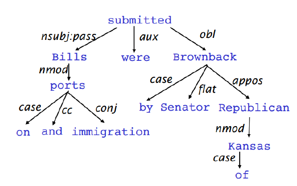
  Dependency tree for the sentence "Bills on ports and immigration were submitted by Senator Brownback, Republican of Kansas" - Source: CS224N

  This is a simple approach (see image below) since it lacks extra nodes for phrasal constituents or lexical categories, making the training of a dependency parser affordable with supervised ML techniques.

  
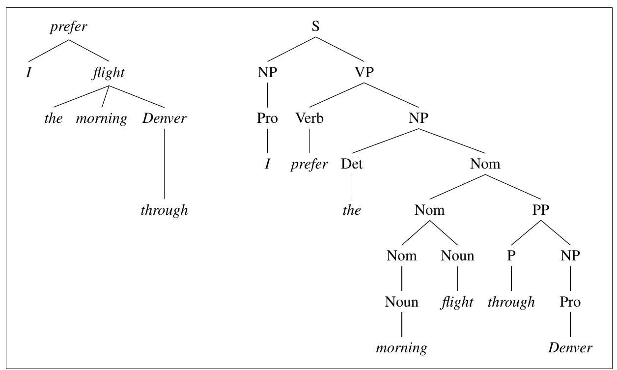
  A dependency-style parse alongside the corresponding constituent-based analysis for "I prefer the morning flight through Denver". Source: Speech and Language Processing by Daniel Jufarsky and James H. Martin

Dependency Parsing

It is the task of analyzing the syntactic dependency structure of a given input sentence $S$. Formally, it wants to create a mapping from the input sentence with words $S = w_0w_1 ...w_n$ (where $w_0$ is the $ROOT$) to its dependency tree graph $G$. The output of a dependency parser is a dependency tree where the words of the input sentence are connected by typed dependency relations (in this case, using the Tesnière convention).

The Dependency Parsing Process

It is composed of two steps:

1. Learning: Given a training set $D$ of sentences annotated with dependency graphs (ground truths), learn a model $M$ to parse new sentences. We can obtain training data from the Universal Dependencies Treebanks, which contains human-annotated dependency trees from several languages.
2. Parsing (inference): Given a parsing model $M$ and a sentence $S$, infer the optimal dependency graph $D$ for $S$ according to $M$.

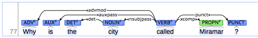
A dependency graph - Source: Universal Dependencies Treebanks

The biggest challenge when doing dependency parsing is dealing with the ambiguities present in our languages.

Dependency Parsing Approaches

Transition-Based Dependency Parsing

It uses a state machine that tells us which possible transitions we can do from the current state. The learning process tries to create a model to predict the next transition based on the transition history. Most transition-based systems do not make use of formal grammar.

Greedy Deterministic Transition-Based Parsing

Joakim Nivre introduced this system in 2003. It commonly uses Support Vector Machines in its implementation. The combination of the stack's status, buffer contents, and dependency relations determine the current state of the parser. An oracle serves as a database to get the transition to make given the parser's current state.

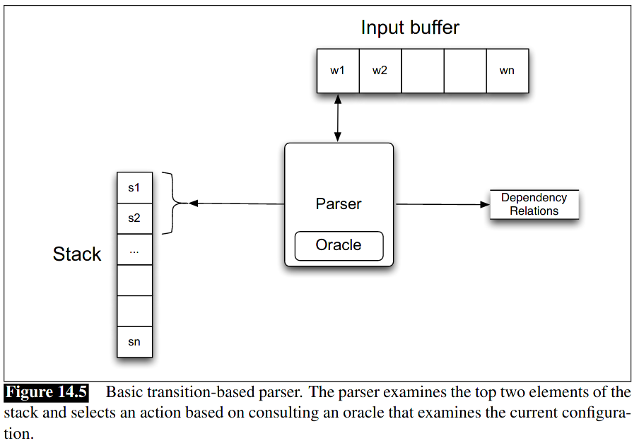
Source: Speech and Language Processing by Daniel Jufarsky and James H. Martin

Greedy, Transition-based Neural Dependency Parsing

In the previous method, we used an oracle to determine the following transition. That oracle contains thousands or millions of rules, something like:

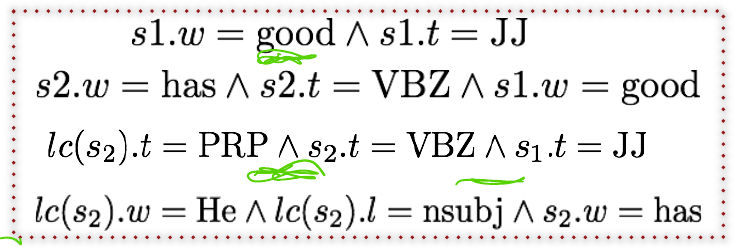
Source: CS224N

Instead of using these error-prone indicator feature databases, we can learn them using a neural network (Chen and Manning, 2014).

This NN model aims to predict a transition sequence from some initial configuration $c$ to a terminal configuration, which encodes the dependency parse tree.

As the model is greedy, it attempts to correctly predict one transition $T ∈ \{shift, Left-Arc_r , Right-Arc_r \}$ at a time, based on features extracted from the current configuration $c = (σ, β, A)$. Where, $σ$ is the stack, $β$ the buffer, and $A$ the set of dependency arcs for a given sentence.

As an example to illustrate how a Transition-Based Parser works, let's analyze the phrase "I ate fish" with the arc-standard system created by Nivre:

1. We have a stack (in grey) and an input buffer (in orange):

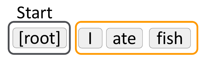
Source: CS224N

2. We are going to move a word from the buffer to the stack. Then we'll query our database to see if there is a dependency for the pair. If there is a match, we'll output the dependency relationship. In our example we proceed like this:

   • Make a shift operation and move I to the stack. We now have two items, we should analyze them with the oracle, but as root is not a word, we do nothing

   
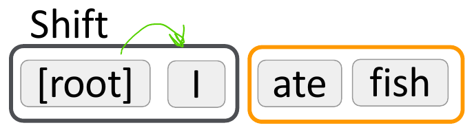
   Source: CS224N

   • Shift ate to the stack and analyze. Now we have two valid words to analyze and when we consult the oracle we know that I depends on ate (I is a noun subject - nsubj of ate), then the relationship is a left arc from the head to the dependent. With this conclusion we add the dependency relationship $A+ = nsubj(ate \to I)$ to our output $A$. Finally, we remove the dependent I from the stack.

   
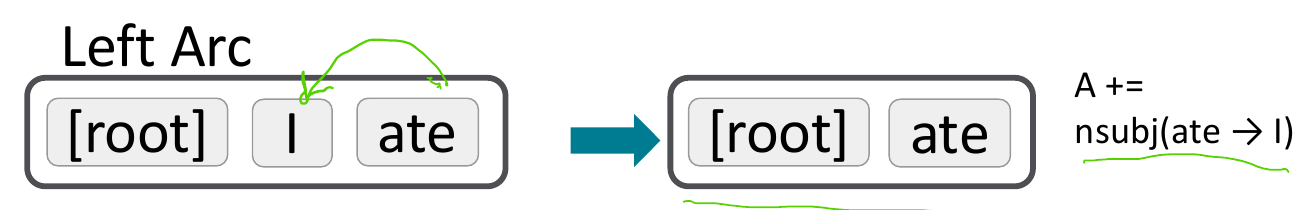
   Source: CS224N

   • Shift fish to the stack and analyze. When we consult the oracle we know that fish depends on ate (fish is the object - obj of ate) then the relationship is a right arc from the head ate to the dependent fish. We add the dependency relationship to $A$: $A += obj(ate \to fish)$ and remove fish from the stack. Notice that now our buffer is empty.

   
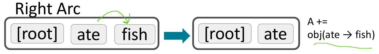
   Source: CS224N

   • Since our buffer is empty, we can analyze the last two items in the stack and add the final dependency relationship.

   
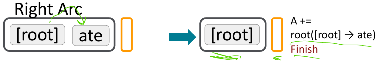
   Source: CS224N

When the algorithm finishes, we have a dependency tree that starts from the root with one child, ate, which has two children, I and fish.

Implementing a Neural Model for a greedy, transition-based Dependency Parser

Now it is time to implement a dependency parser following the paper by Chen and Manning, 2014.

Inputs

We'll use dense vector representations of the current state (feature set). The vector can include words, dependency labels (for example, NNS for plural nouns, nummod for numerical modifiers, etc.), and part-of-speech tags (POS). All of the selected features are concatenated into a large input vector and feed to the neural network.

NN Architecture

We'll use a simple feed-forward neural multi-class classifier as described below:

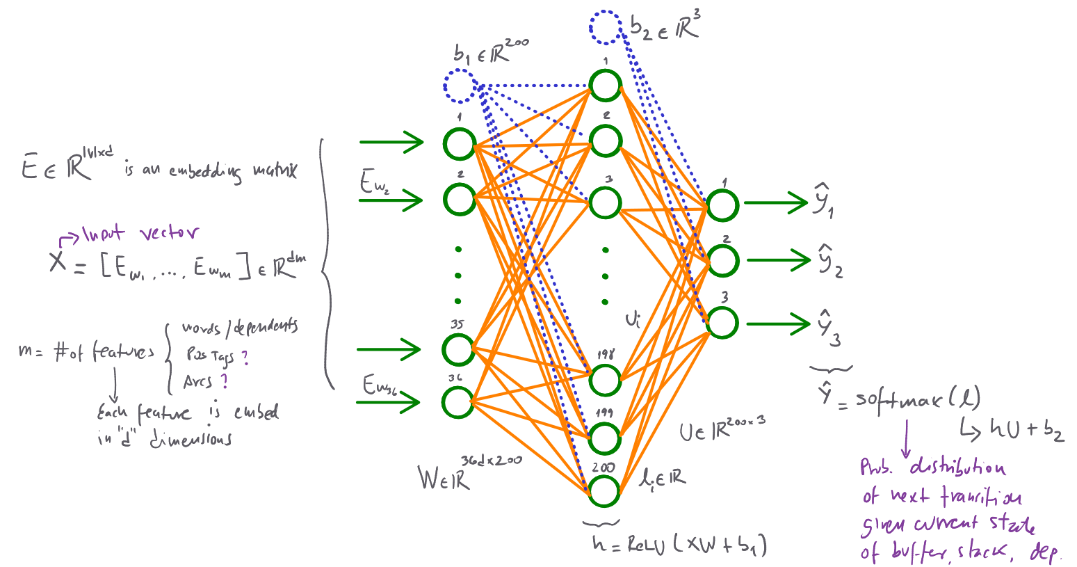
Source: Own

Training Process

1. Extract the features vector representing the current state $w = [w_1, w_2, \dots , w_m]$ where $m$ is the number of selected features, and $w_i$ is the index of the token associated with the $i$-th feature.
2. Look up the embedding matrix $E \in \R^{|V| \times d}$ for each element in $w$. This will produce a vector $x = [E_{w_1}, E_{w_2}, \dots, E_{w_m}] \in \R^{dm}$ where $E_{w_j}$ is an embedding for the token associated with feature $j$. Notice we make this lookup in minibatches, then we'll have $w_{batch} \in \R^{batch\_size \times m}$ and $x_{batch} \in \R^{batch\_size \times dm}$.
3. Compute the forward pass with:
   $$\begin{aligned} h &= ReLU(xW + b_1) \\ l &= hU + b_2 \\ \hat{y} &= softmax(l) \end{aligned}$$
   where:
   • $W \in \R^{36d \times 200}$
   • $U \in \R^{200 \times 3}$
   • $b_1 \in \R^{200}$
   • $b_2 \in \R^{3}$
4. Update the parameters with:
   $$\begin{aligned} J(\theta) = CE(y, \hat{y}) = - \sum_{i=1}^3y_i \log \hat{y_i} \end{aligned}$$
   Where $CE$ is the Cross Entropy Loss.

Implementation notes

Please refer to this repository to check the entire code of the implementation. In this section I want to share some important notes about it:

• We are using the Xavier initialization for the weight matrices and the Uniform initialization for the bias vectors

• Even if PyTorch provides an embeddings layer we choose to implement this from scratch. It is interesting to understand how we can achieve it with provided methods in the library avoiding expensive for-loops in the process:

  1. As at the end we'll have a large input vector we can flatten $w_{batch}$ with the flatten method.
  2. We can use the flatten vector $w$ to select the items in the embedding matrix $E$ using the convenient index_select method.
  3. As we need a tensor to input the minibatch embeddings we can reshape the output of the previous step with the view method to obtain a $batch\_size \times dm$ matrix.

  The resulting snippet is:

  x = torch.index_select(self.embeddings, 0, torch.flatten(w)).view(
            w.shape[0],
            self.n_features*self.embed_size
            )

• To avoid overfitting we are going to use a dropout layer with a default dropout probability of 50%. PyTorch provides a dropout layer that can be initialized with nn.Dropout(self.dropout_prob). Later, during the forward pass (dropout layer turned on with parser.model.train()), we embed the hidden layer into the dropout layer letting PyTorch taking care of turning the units on/off. So convenient!

• During training we used the Adam optimizer with default parameters ($\beta_1 = 0.9, \beta_2 = 0.999$, and $\epsilon = 10^{-8}$) and a learning rate of $0.0005$. This can be constructed with optim.Adam(parser.model.parameters()).

• We trained the model with 10 epochs and a minibatch size of 1024.

• The UAS metric was used to track the progress of the model. The value of this metric was evaluated after each epoch (dropout layer previously turned off with parser.model.eval()) with the Dev data set.

Training results

The training process just took less than 12 minutes and I got great results as shown below.

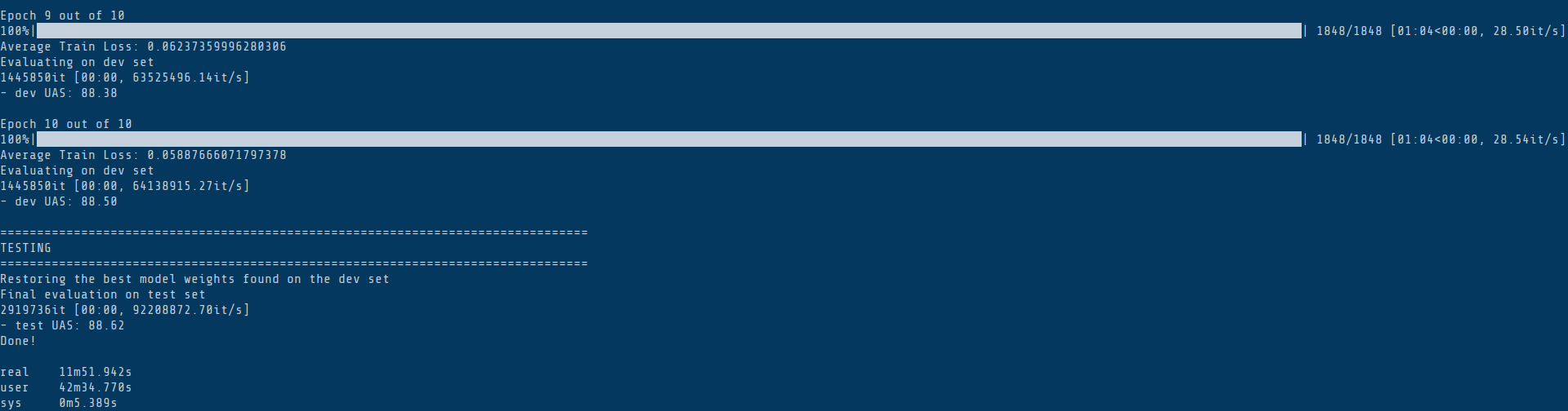
Source: Own

No todo es color de rosa

Or, "not everything is peaches and cream". There are cases where our neural parser might get the dependencies wrong. In general, the parsing error types can be categorized into four groups:

1. Preposition Phrase Attachment Error
2. Verb Phrase Attachment Error
3. Modifier Attachment Error
4. Coordination Attachment Error

In all the above cases the head-words are wrongly chosen. In the Coordination Attachment Error, it is important to mention that the second conjunct should be attached to the first conjunct and not the other way around. For example:

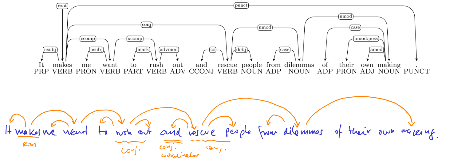
Source: CS224N/Own

The parser returned the dependency $makes \to rescue$ which is incorrect. It should be $rush \to rescue$

We can improve the UAS metric by tunning the hyperparameters, adding more training samples of these special cases, or checking our overfitting status.

What does the future hold?

As always thanks for your time, hope you find the article useful. Working on the neural dependency parser is a nice introduction to NN with PyTorch, and from now on, I'm thrilled to know that complex NN architectures (to solve complex tasks) are just around the corner!

Source: xkdc

Have a great rest of your day!