Hello, welcome to this new chapter in my exploration of NLP. This time I review a practical application: Neural Machine Translation (NMT). NMT also introduces us to complex neural network architectures like Recurrent Neural Networks and sequence-to-sequence models.

In this post, I will discuss how an NMT works. How to train it, and how to infer from the model once we obtain its parameters.

It is a long article, so without further ado: Let's get started!

Table of Contents

• A brief history of machine translation

  • Alignment

• Black-boxes to the rescue

  • The architecture behind NMT: Seq2seq or Encoder-Decoder models

    • Encoder
    • Decoder

  • Inferring from a seq2seq model

  • Attention to improving seq2seq NMT

• NMT training with PyTorch

  • Understanding the architecture and dimensions

  • The equations for an NMT model with Attention

    • The Encoder's hidden and cell states
    • The Decoder's initial hidden and cell states
    • The Decoder's following hidden and cell states
    • The Decoder's next prediction

  • The model's Loss Function

  • Working with Batches

  • Managing Embeddings

  • Packing padded sequences

  • Encoding

  • Decoding

• Evaluating NMT

• Training results

• Universal Translator: Are we there yet?

A brief history of machine translation

Until about 2010, computer translations used statistical models with parallel corpora (i.e., manually created input datasets in the source and target language). The outputs of this type of model were not good (I think we all remember those days). However, in 2014 neural networks started to be used, specifically Recurrent Neural Networks (RNN) through an architecture called seq2seq (sequence-to-sequence). Since then, this type of architecture has become popular due to its simplicity comparing to statistical translation models and its good results.

Alignment

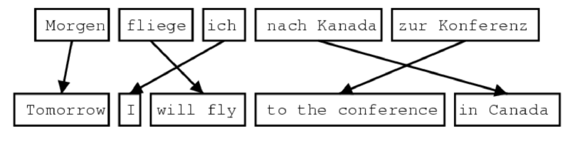
Statistical translation attempts to learn a model $P(y|x)$ from a parallel dataset. For this purpose, we add (without being explicitly specified in the data) a latent variable $a$ called alignment to consider the word-level correspondence between the source sentence $x$ and the target sentence $y: P(y, a|x)$.

Learning the alignment between the two sentences is a complex task that required most of the computational effort in this type of translator.

Alignment relationships can be one-to-one, one-to-many, many-to-one, and many-to-many. Source: CS224N.

Black-boxes to the rescue

Instead of defining rules to identify the alignments, it is possible to train an NN to learn them implicitly, and given the results, this method performs very well. All we need is a huge dataset and many GPUs :)

The architecture behind NMT: Seq2seq or Encoder-Decoder models

The sequence-to-sequence models are best suited to capture long-term dependencies in comparison to probabilistic models. And this is probably one of the reasons for their success.

These end-to-end models consist of two components:

• An Encoder: In charge of taking the input sequence and returning a fixed-size encoded context vector.
• A Decoder: In charge of generating an output sequence using the Encoder's context vector as input seed.

In both cases, the inputs for the Encoder and Decoder are word embeddings (we can use pre-trained word vectors like GloVe or word2vec, or learn them during the NMT training process). An NMT model also defines a couple of vocabularies. One for the source language and another one for the target language.

Encoder

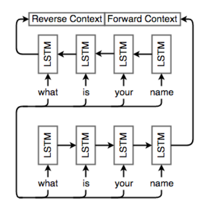
Performs its job by using a Recurrent Neural Network (commonly an LSTM or Long Short-Term Memory). As the dependencies in sentences work either from left-to-right and right-to-left, it is common to use a bidirectional LSTM to capture them.

A single-layer bidirectional LSTM Encoder network. Source: CS224N

Decoder

It also uses an LSTM network and acts like a conditional language model since its predictions depend on the Encoder's output.

Inferring from a seq2seq model

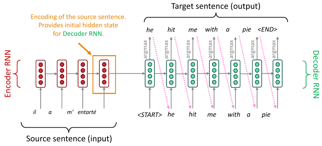
A simple seq2seq model for NMT during test time. Source: CS224N

In the image above, the model tries to predict the conditional probability of the target sentence $y$ given a source sentence $x$. This approach means we want to produce the sequence of words that make $y$ to have the highest probability.

As the search space can be enormous (on each time step $t$ of the decoder, we are tracking $V^t$ possible combinations, where $V$ is the vocabulary size), we need to use a technique to reduce it. One easy option is to select the most probable ($argmax$) token from the output vocabulary at each time step (Greedy Decoding). But choosing like this doesn't guarantee the best translation. Furthermore, once we made a mistake, there is no way to go back and fix it.

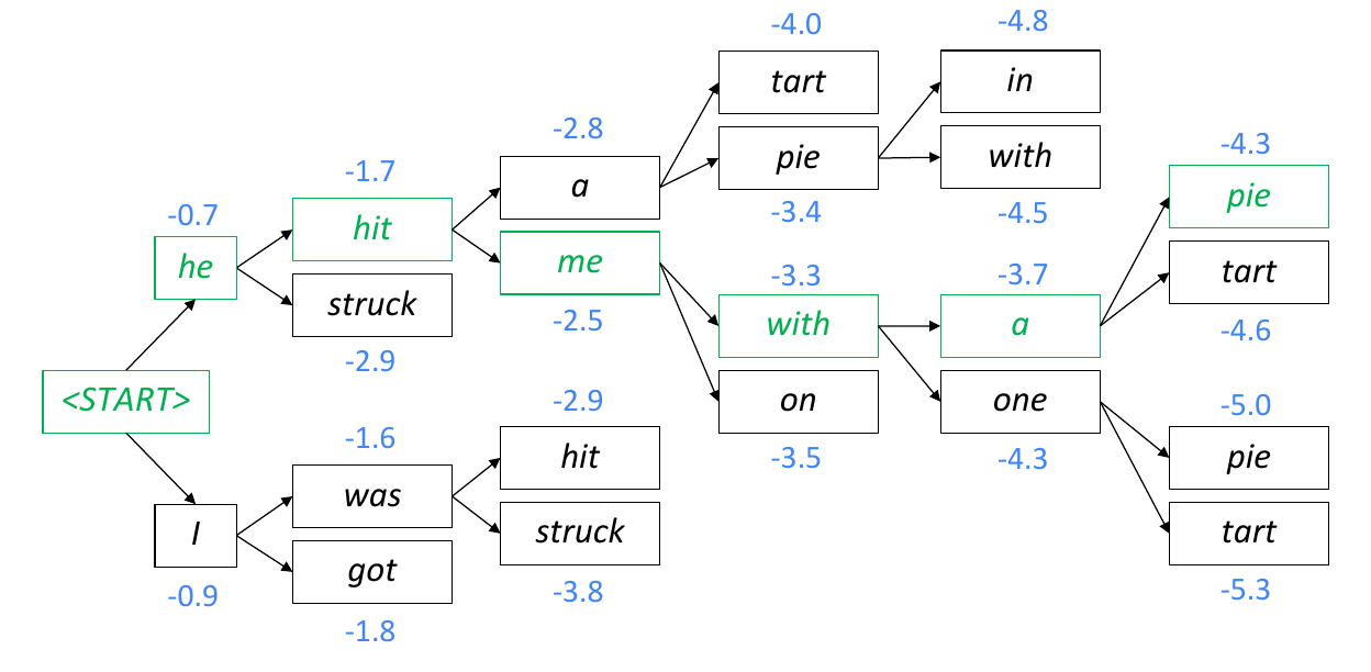
For this reason, it is better to choose a local search approach, like Beam Search, where we maintain $K$ candidates or partial translations (hypotheses).

Each hypothesis $y_1, \dots, y_t$ has a score. We choose the higher one among the candidates:

An example of Beam Search Decoding. At each step, we expand the K-nodes with the highest value. When we finish, we backtrack starting from the last-level node with the biggest value. Source: CS224N

Note: Greedy Decoding is a particular case of Beam Search when $K = 1$.

In Greedy Decoding, we decode until the model produces an <END> token. In Beam Search Decoding, different hypotheses may output <END> tokens on different timesteps. When a hypothesis produces an <END> token, we mark it as complete, place it aside, and continue exploring other hypotheses via Beam Search.

CS224N

We keep doing Beam Search until:

• We reach timestep $T$ (a pre-defined cutoff), or
• We have at least $n$ completed hypotheses (where $n$ is pre-defined cutoff)

When we finish the search, we would have a list of completed hypotheses. As shorter hypotheses will have higher scores, we need to normalize the values by length and select the biggest one:

One disadvantage with Beam Decoding is that it doesn't guarantee finding an optimal solution. Nevertheless is much more efficient than an exhaustive search and provides good results.

Attention to improving seq2seq NMT

It is not enough to use a bidirectional Encoder connected to an LSTM Decoder with Beam Search to have good results.

As we rely on the last output vector in the Encoder component we are hoping all context and most important information from the full source sentence to be encoded in it, but this might not be true. We refer to this as information bottleneck.

CS224N

Attention solves information bottleneck by using a direct connection from the Decoder to the Encoder to focus on particular elements of the source sequence at every decoding step. This technique allows the Decoder to decide what input words are the most important ones at any point in time.

We compute the Attention calculations like this:

1. Compute the Attention scores for the Decoder's step $t$ for all Encoder's hidden states ($m$):
   $$\begin{aligned} e_{t,i} = (h_t^{dec})^TW_{attProj}h_i^{enc} \text{ where } e_t \in \R^{m \times 1}, W_{attProj} \in \R^{h \times 2h}, 1 \leq i \leq m \end{aligned}$$
2. Calculate the Attention distribution:
   $$\begin{aligned} \alpha_t = Softmax(e_t) \text{ where } \alpha_t \in \R^{m \times 1} \end{aligned}$$
3. Get the Attention output:
   $$\begin{aligned} a_t = \sum_i^m \alpha_{t,i}h_i^{enc} \text{ where } a_t \in \R^{2h \times 1} \end{aligned}$$

We then use $a_t$ to calculate the Decoder's prediction and influence on the prediction of the next decoding step during training.

NMT training with PyTorch

Now it is code time! As usual, you can check the full implementation on this repository.

In general, we use the same approach we followed when training the Neural Dependency Parser:

• Define a Loss Function $J$.
• Minimize $J$ with SGD and backpropagate (in this case, Backpropagation Through Time).

As we are using two networks (Encoder and Decoder), we choose to train them simultaneously to learn the same context vector representation.

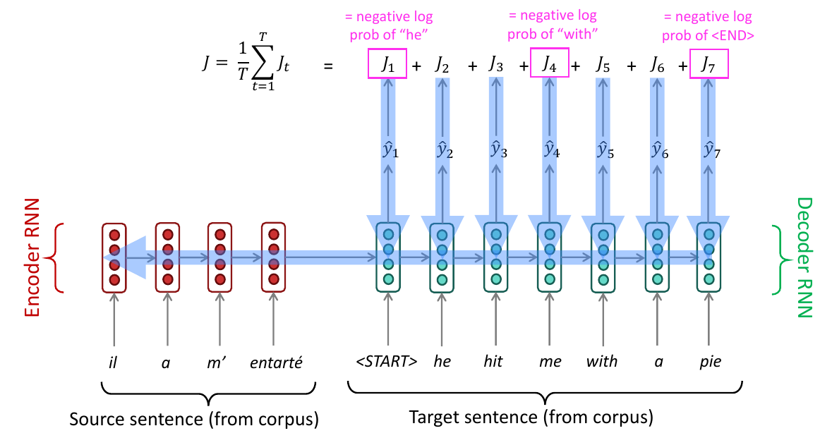
A simple seq2seq model for NMT during training. Source: CS224N

In the following sections, I want to share some notes that helped me when implementing the NMT.

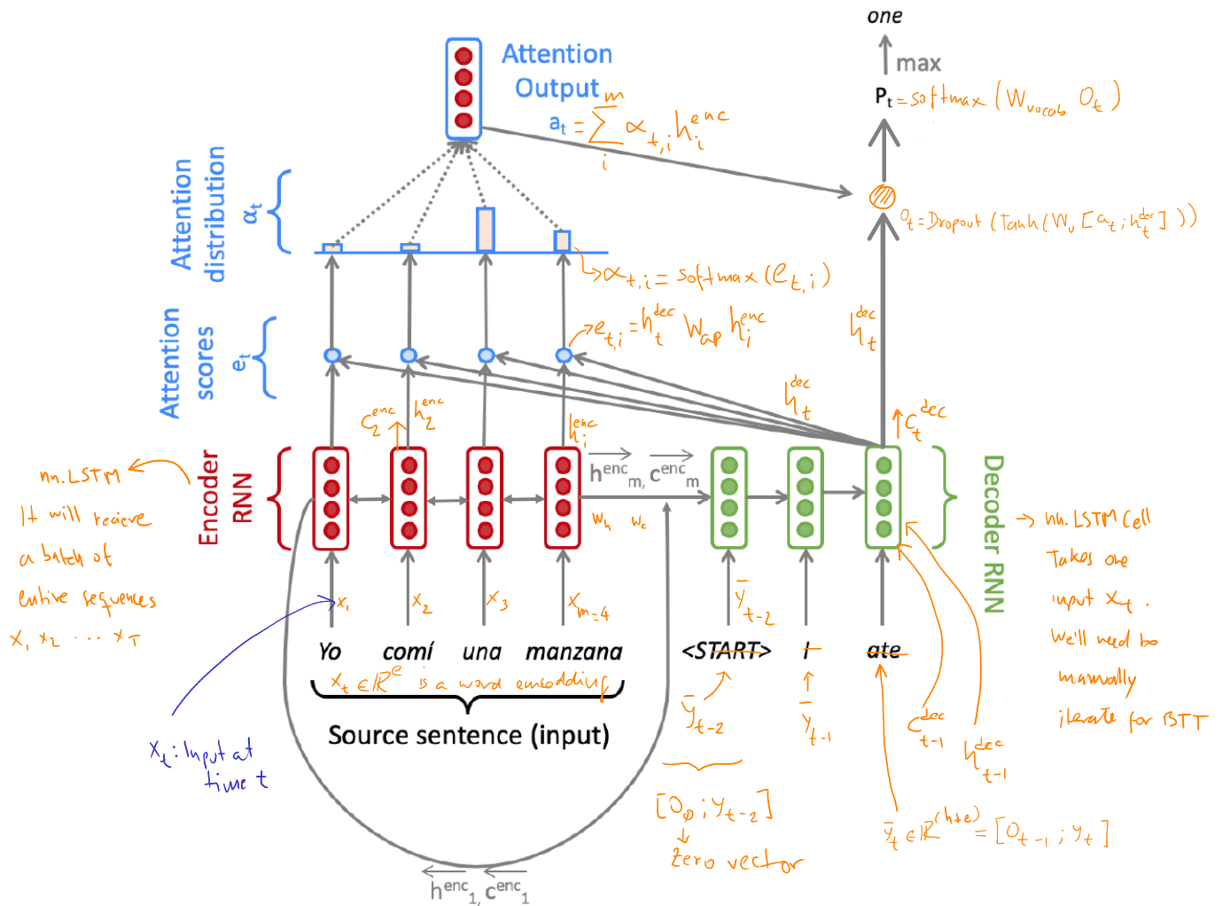
Understanding the architecture and dimensions

A seq2seq model with Attention for NMT during training.

The equations for an NMT model with Attention

The Encoder's hidden and cell states

The Decoder's initial hidden and cell states

The Decoder's following hidden and cell states

Where $\bar{y_t}$ is the concatenation of $y_t$ (corresponding word of a matching sentence in the target language) with the combined-output vector $o_{t-1}$ from previous timestep.

The Decoder's next prediction

Where $V_t$ is the target vocabulary size and $h$ is the hidden size, which in this case is equal to the embedding size.

The model's Loss Function

Where $g_t$ is a one-hot vector of $y_t$.

Working with Batches

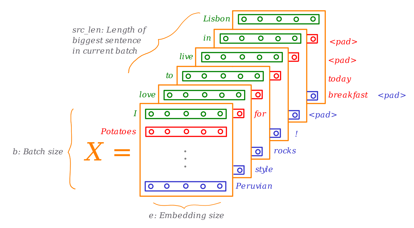
We want to train the model with batches composed of sentences where each sentence is a sequence of words (actually word embeddings). But as we need a fixed size input for all the sentences in the batches, we first need to pad the shortest sentences until all have a length equal to the maximum sentence length in the batch.

Note: Remind the location of the pad token in our vocabularies since we'll need it later during training.

Since we need to work with numbers instead of strings, we use matrices for the source and target batches with integer indexes that indicate the string location in the vocabularies objects. This means that, so far, our input/output batches' shapes are something like $(src\_len, b)$ where $src\_len$ is the length of the longest sentence in the batch, and $b$ is the batch size.

Wait a minute. Shouldn't it be more intuitive to represent the input batch with a shape of $(b, src\_len)$? Probably yes. But it seems PyTorch methods expect as input a tensor where the first element is not the batch size (by default). For example, rnn = nn.LSTM(10, 20, 2) defines an LSTM layer with input_size = 10, hidden_size = 20, and num_layers = 2. The input of this layer (contains the features of the input sequence) should have a shape of $(L=src\_len,N=b,H_{in}=10)$ when the optional parameter batch_first=False (this is the default value) or $(N, L, H_{in})$ when batch_first=True.

Notice how in the previous example, the parameters defining the LSTM don't relate with the input elements except for the hidden size of the LSTM cells, which in our case is the embedding size.

Managing Embeddings

As I mentioned before, we have two alternatives: Use pre-trained embeddings like GloVe or word2vec, or learn them using our NMT dataset while we train our NMT with PyTorch's nn.Embedding layers.

How PyTorch learns these embeddings? Which algorithm uses? Those are excellent questions for which I don't have answers yet.

Anyway, we can use the PyTorch embedding layers as lookup tables to get the word vectors given a tensor with the word indexes we want to retrieve.

For example, we can define two embedding layers, one for the source language and the other for the target language, like this:

class ModelEmbeddings(nn.Module):

  def __init__(self, embed_size, vocab):
    # [...]
    src_pad_token_idx = vocab.src['<pad>']
    tgt_pad_token_idx = vocab.tgt['<pad>']

    self.source = nn.Embedding(len(vocab.src), embed_size, src_pad_token_idx)
    self.target = nn.Embedding(len(vocab.tgt), embed_size, tgt_pad_token_idx)

When we later want to get the embeddings, we can query for them like this - notice the shape of source_padded is $(src\_len, b)$:

X_embeds = self.model_embeddings.source(source_padded)

Now we have an extra dimension (the embedding's size), and the resulting tensor might be complex to visualize. For me, this looks like this:

A visualization of an NMT model's inputs. Source: Own

Packing padded sequences

Padding helps us ensure we have the same length for all our input sequences, but the added padding tokens don't provide information for the model training. They increase our model's training computation cost as explained here.

Fortunately, PyTorch provides a way to dealing with this: packing the padded sequences with the method pack_padded_sequence.

Once we pack our input tensor, we can use it to feed a layer or make calculations. The output of these operations will output packed values that can be unpacked with the pad_packed_sequence method.

Knowing this, we can feed our LSTM's Encoder in this way:

class NMT(nn.Module):

  def encode(self, source_padded: torch.Tensor, source_lengths: List[int]) -> Tuple[torch.Tensor, Tuple[torch.Tensor, torch.Tensor]]:

    # [ ... ]

    # 1. Constructing X
    X_embeds = self.model_embeddings.source(source_padded)  # This adds e to the shape
    X = pack_padded_sequence(X_embeds,source_lengths)

    # 2. Encode the batch
    enc_hiddens, (last_hidden, last_cell) = self.Encoder(X)  # h_0, c_0 default values are zeroes
    enc_hiddens, output_lens = pad_packed_sequence(enc_hiddens)
    enc_hiddens = enc_hiddens.permute(1, 0, 2)

Read here for more information about how packing/unpacking works in PyTorch.

Encoding

This is done by the encode method. It converts the padded source sentences (source_padded) into the tensor $X$, generates $h^{enc}_1 , \dots , h^{enc}_m$ as enc_hiddens, and computes the initial state $h_0^{dec}$ (init_Decoder_hidden) and initial cell $c_0^{dec}$ (init_Decoder_cell) for the Decoder.

Decoding

The decode method constructs $ȳ$ and runs the step function over every timestep for the input.

We first need to prepare the inputs for the Decoder. We do this in the final part of the Encoder process since its last hidden state and cell are the inputs for the Decoder's initial state - equation $(2)$, let's remember how these elements look like:

As you can see, we need to make a linear projection with the last elements of the Encoder. We already defined a linear layer for this when initialized the NMT class:

class NMT(nn.Module):
    def __init__(self, embed_size, hidden_size, vocab, dropout_rate=0.2):
	
	# [ ... ]

	self.Decoder = nn.LSTMCell(
            input_size=embed_size+embed_size,  # !! This is \bar{y}_t
            hidden_size=hidden_size,
            bias=True
        )

	# Linear projection with W_{h}
        self.h_projection = nn.Linear(
            in_features=hidden_size*2,  # We receive [h_1 <-; h_m ->]
            out_features=hidden_size,  # We obtain a hidden-size vector
            bias=False
        )

        # Projection with W_{c}
        self.c_projection = nn.Linear(
            in_features=hidden_size*2,  # We receive [c_1 <-; c_m ->]
            out_features=hidden_size,  # We obtain a hidden-size vector
            bias=False
        )

Notice the Decoder is an LSTM cell, not a layer. Since we won't work with batches in the Decoder, we need to add a loop to process the sequences and apply the Attention calculations.

Before applying the projection, we need to concatenate the last hidden/cell vector's outputs from the left-to-right and right-to-left passes of our Encoder (remember it is a bidirectional LSTM). Recall the Encoder returned the last hidden/cell values into last_hidden and last_cell, and both variables' shape is (2, b, h). Then we can get the final values of the last hidden and cell with:

class NMT(nn.Module):
    def encode(self, source_padded: torch.Tensor, source_lengths: List[int]) -> Tuple[torch.Tensor, Tuple[torch.Tensor, torch.Tensor]]:

	# [ ... ]

	# 3. Compute the Decoder initial state
        # init_Decoder_hidden
        last_hidden_flat = torch.cat((last_hidden[0], last_hidden[1]), 1)
        init_Decoder_hidden = self.h_projection(last_hidden_flat)

        # init_Decoder_cell
        last_cell_flat = torch.cat((last_cell[0], last_cell[1]), 1)
        init_Decoder_cell = self.c_projection(last_cell_flat)

        dec_init_state = (init_Decoder_hidden, init_Decoder_cell)

last_hidden[0] represents the left-to-right pass of our bidirectional LSTM. Also, notice these linear layers will learn the parameters $W_c$ and $W_h$. The second parameter in the cat method means to add the second vector as a column of the first one.

Evaluating NMT

We use the BLEU (Bilingual Evaluation Understudy) score, which compares the machine-written translation to one or several human-written translation(s), and computes a similarity score based on:

• $n$-gram precision (usually for 1, 2, 3 and 4-grams). This means we are going to compare how many of the $n$-grams that appeared in the NMT also appear in the human translation(s).
• Plus a penalty for too-short system translations

BLEU is useful but imperfect:

• There are many valid ways to translate a sentence
• So a good translation can get a poor BLEU score because it has low $n$-gram overlap with the human translation

Training results

The model was trained with a parallel corpus of more than 200k sentences in Spanish with their corresponding human translations into English. It took about 4.5 hours using an Azure GPU VM with the following characteristics:

• 6 vCPUs with 56GiB RAM
• 1 NVIDIA Tesla K80 GPU with 12GiB RAM
• 150 GiB of SSD storage
• Linux Ubuntu 18.04

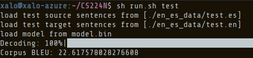
The training process needed 13 epochs and 88k iterations. After training, I tested the model getting a BLEU score of 22.6

Model's training results. Source: Own

Universal Translator: Are we there yet?

Not even close! Machine translation is a complex task. Top-notch translators like Deepl (which, by the way, uses CNNs!) have been trained with millions or perhaps billions of sentences and are adjusted constantly to achieve excellent performance. Regarding this experiment, the results are acceptable considering the dataset size:

I recall that Star Trek episode when Hoshi Sato explains that even with 22nd-century translators, they still require human intervention:

Human translators and interpreters, in my opinion, are still safe for at least a decade. If one of them is reading this article, let me tell you I admire your skills!

As always, thanks for your time reading this. I hope it was helpful. Stay tuned for more NLP experiments coming in the following weeks! 👋