I was wondering how much time I have spent studying and learning. Let's do a crude calculation:
- Pre-school, elementary school, high school, college ~ 17 years.
- Languages ~ 2 years
- Extension courses and certifications ~ 2 years and counting.
- In-house courses ~ 1 year
- Interesting reads from my newsfeed ~ 2 years and counting.
- Other: Music, DIY stuff, cooking, baking, sports, nutrition, health, meditation, etc. ~ 5 years and counting
Wow, that's ~43 of my life, so much time.
If I subtract activities not associated with my career (Computer Sciences), what percentage of study time I spent putting learned theory into practice? Difficult to answer. I remember eminently practical courses such as physics and chemistry labs in college, I also remember extension courses such as computer assembly, but little else comes to mind.
When I talk about time spent in hands-on learning, I am not referring to time as an employee in some company, but the time before being hired (or working on your project if you are an entrepreneur) while finishing your studies.
I venture to say that the time spent in theory will have represented 70% of the total (~7 years!), and the time spent in practice 30%. I am not considering homework or exams. For me, they represent part of the same theoretical learning process.
Would I have liked to reverse these percentages? I don't think so. In any case, I would have preferred to bring them to 50%-50%. But apparently, the educational system that I have had to experience has a preference for theory, and I haven't known any other way of learning so far.
I have been studying AI for almost a year now. I have learned so many things. But some of that knowledge is still connected by weak theoretical threads and even assumptions (will it be the limits of learning?). However, when faced with the challenges of solving a real problem, many of those "weak" areas have been strengthened, connections have grown, new questions have emerged. But most of all, I have been filled with a sense of satisfaction as I noticed how various concepts settled harmoniously in my head.
Right now, I find myself in this sweet stage of practicing what I have been studying in the last few months. I could say it's a similar feeling to what I read on a zen website: watching the snowflakes fall and melt into a uniform whole. It's a happy time, and I want to continue to enjoy this moment as much as I can.
As I thought about all this, the concept of tempering came to my mind:
Tempering is a process of heat treating, which is used to increase the toughness of iron-based alloys.
Wikipedia
In my experience, the word tempering describes this stage of learning very well. And although I did not rank in the top 20, I did manage to be in the top 14%. For me, at this point, that's enough, and now I can continue to explore other practical applications more akin to my interest.
Ok, now let's get to the exciting content. In this article, I share my impressions of Kaggle and its competitions and write down the topics that strongly resonated with me for future reference.
Let's get started!
Table of Contents
Kaggle and Kaggle Competitions
I heard of this platform some months ago, and I categorized it as free GPU, but it is much more than that! According to Wikipedia:
Kaggle, a subsidiary of Google LLC, is an online community of data scientists and machine learning practitioners. Kaggle allows users to find and publish data sets, explore and build models in a web-based data-science environment, work with other data scientists and machine learning engineers, and enter competitions to solve data science challenges.
Kaggle is an excellent idea to boost the ML field, ultimately a win-win for everyone involved. Regarding the competitions, some of them are oriented to learn, and others to earn money. In the latter, the "host pays the prize money in exchange for a worldwide, perpetual, irrevocable and royalty-free license [...] to use the winning Entry ".
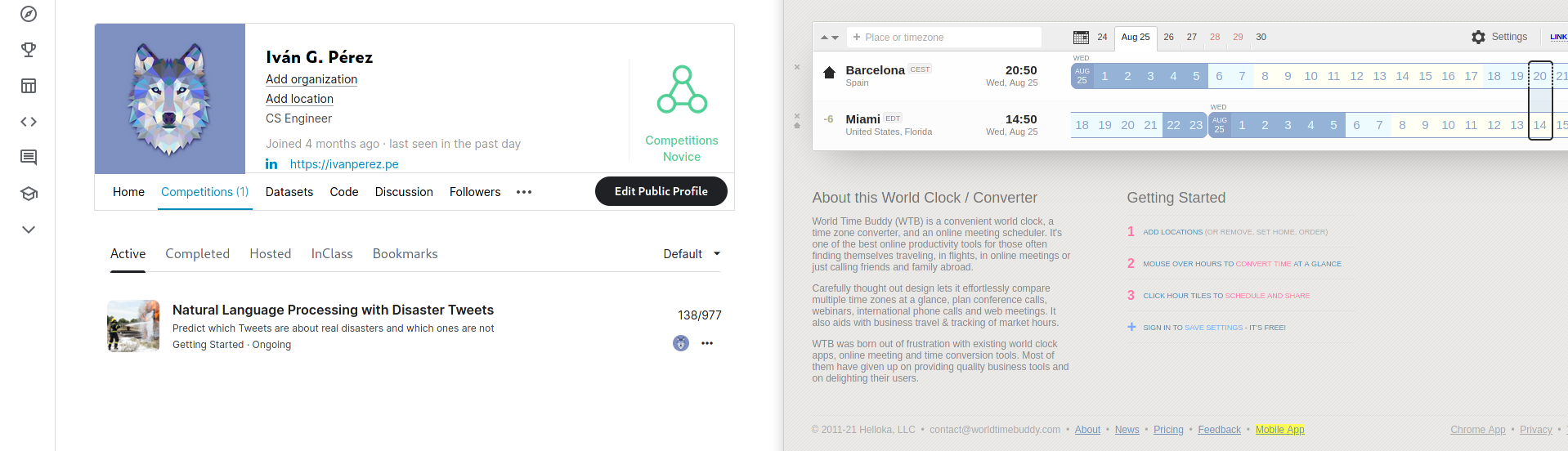
In my case, I am interested in learning competitions. I decided to start with something basic in NLP: identify which tweets refer to a disaster and which do not.
This competition is about a simple binary classification problem. The idea is to achieve the highest possible score using the test dataset provided by the organizers. The first thing that caught my attention was seeing many people on the leaderboard who achieved a perfect score, getting 100% of the predictions right. Surprising? Yes, realistic? I'm not sure. I found out later that someone found the test dataset with the True labels and that several people used it to achieve perfect scores and appear in the first positions. It is sad to know this, but hey, everyone is free to make their own decisions and do what they believe is the best for themselves. In my case, my goal is to learn and knowing this, I started to read the leaderboard differently, and I downplayed it.
Experiment? How?
Unlike other fields where solving a problem is a deterministic activity. In ML, we need a different approach due to the large number of hyperparameters. Solving an ML problem becomes an iterative activity that requires a methodology. You should be orderly, write down the changes, the reasons for making them, and the results obtained. Likewise, it is necessary to use metrics to determine if the changes improve or worsen the predictions of our models. In short, we need to apply the scientific method:
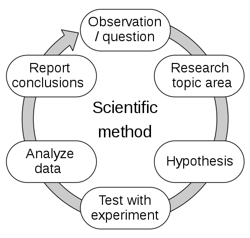
Source: Wikipedia
Chapter 11 of "Deep Learning" by Goodfellow, Bengio, and Courville may serve as an introduction. I have not had a chance to research other methodological approaches to ML practice, but I put it on my to-do list.
For the moment, and to begin with, I will use a set of simple rules:
- Build a simple model as quickly as possible.
- Train the model and take note of the metrics obtained in the first run. The values obtained will serve as a baseline to determine if subsequent changes represent improvements to the initial model.
- Make only one change at a time and after implementing it, take note of the resulting metrics, compare them with the previous ones and decide whether to incorporate the change or not.
- Once the possibilities of changes are exhausted, commit the kernel and send the result to obtain the final score.
An optimization problem inside of an optimization problem?
After establishing the parameters for the experimentation, it is time to go to the resolution of the problem itself. In this case, understanding the problem is simple, so we can move on to the next point: with what architecture do I solve the problem? What algorithm/model do I use? There are many options! Which to choose?
I would have to try all of them to determine which one best suits my need, but I don't have the resources to do it. There must be another way. I add on my to-do list: Research on "model/algorithm selection". For now, I will use my intuition.
I tell myself that for the best results, I should use a SOTA model. Although it is better to start with something simpler and see how good results I can get. Let's start then with a BiLSTM.
I ask myself: Choosing the best architecture/model/algorithm/hyperparameters is an optimization problem? If I see it as maximizing the accuracy of the model's predictions while minimizing the computational cost of training, yes, indeed, it looks like an optimization problem 😵💫.
EDA
Without further delay, I started coding a BiLSTM with TensorFlow, and realized that I was missing the most important thing of all, the data! This omission serves me as an excellent lesson: Always start with the data. Always.
We can accomplish this task with the Exploratory Data Analysis (EDA), which requires a separate article that I will love to write once I know more about it. I add another item to my to-do list.
On this occasion, I just did a naive EDA focusing my attention to determine whether the data was balanced or not.
While looking for information, I found an excellent Google article describing some relevant ratios/metrics for the text classification problem and proposing an algorithm to determine which model to use. How did they get it? With many resources!:
We ran a large number (~450K) of experiments across problems of different types (especially sentiment analysis and topic classification problems), using 12 datasets, alternating for each dataset between different data preprocessing techniques and different model architectures. This helped us identify dataset parameters that influence optimal choices.
Google
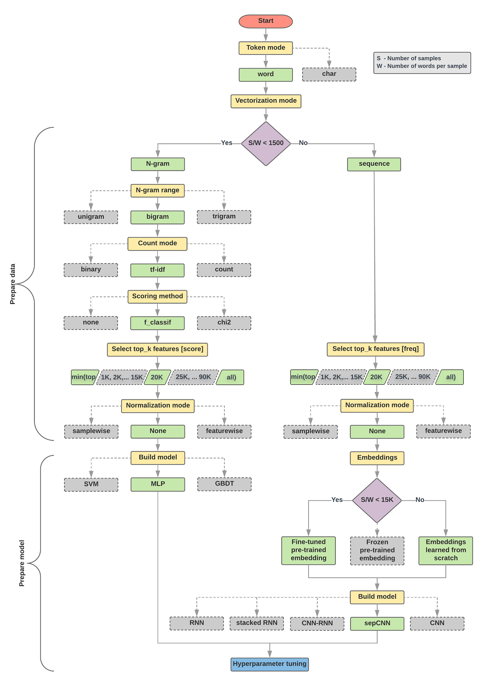
Source: Google's Machine Learning Guide for Text Classification
The flowchart above was very helpful in determining my next steps:
- Calculate the ratio WS where S is the number of samples and W is the number of words per sample. According to Google's experiments, this ratio has the highest correlation with the model choice for this type of problem.
This is very important and probably applies to other types of problems in ML (maybe all of them): Study the training dataset to determine the best model/algorithm to use, or at least, to build intuition.
- After testing with an RNN, solve the problem with an MLP (the WS ratio for this competition's dataset was <1500 ). Why not start with an MLP? Because an RNN is easier to implement in TensorFlow, also I wanted to give it a chance while practicing coding in TensorFlow.
- After MLP, try a Transformer.
First try: Solve the challenge with an RNN
The training dataset looks like this:
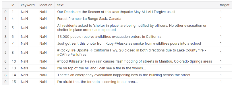
Source: Kaggle
As I wanted to make a super simple baseline:
- I didn't preprocess the data. I only replaced the
np.nan values with empty strings.
- I didn't use a validation dataset. I split the training data into training and test sets (80-20). For validation, I used the test set.
- I concatenated the keyword, location, and text columns into a single column using a comma as a separator. I used the concatenated text as training examples.
- I used the default Keras "
TextVectorization layer" to vectorize the training examples.
- I learned the 64-dimensional word embeddings from scratch using the
tf.keras.layers.Embedding layer with masking to handle the variable sequence lengths.
- To enrich the embeddings encoding, I used a bidirectional LSTM.
- The output came out after a
Dense layer without dropout for the moment.
model = tf.keras.Sequential([
encoder,
tf.keras.layers.Embedding(input_dim=len(encoder.get_vocabulary()), output_dim=64, mask_zero=True),
tf.keras.layers.Bidirectional(tf.keras.layers.LSTM(64)),
tf.keras.layers.Dense(64, activation='relu'),
tf.keras.layers.Dense(1, activation="sigmoid")
])
On regards the optimization process:
BinaryCrossentropy as loss.Adam optimizer with LR of 1e−4.accuracy as metric.
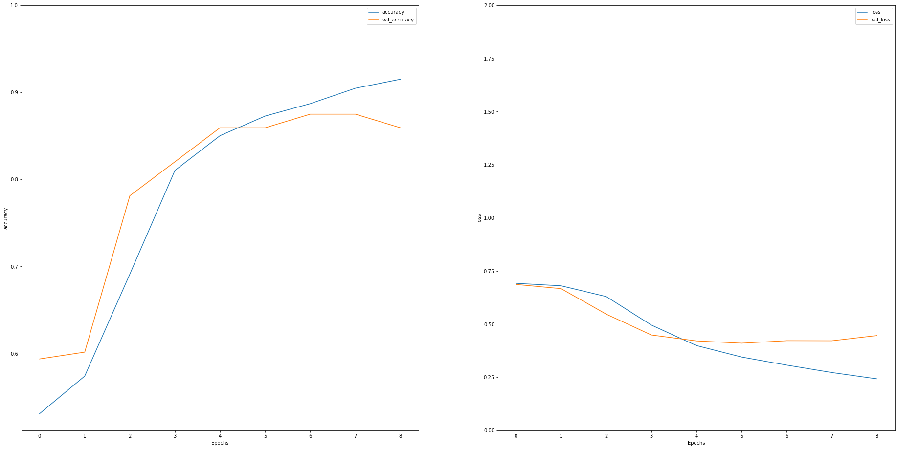
After running the training process several times (re instantiating the model object each time), I saw signs of overfitting after ten epochs, so I stop the training at that time. The results were like this:
24/24 [==============================] - 0s 11ms/step - loss: 0.4705 - accuracy: 0.7919
Test Loss: 0.47046178579330444
Test Accuracy: 0.7918581962585449
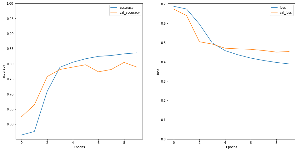
Source: Kaggle, own.
Not that bad, right? When submitting the prediction results to the competition, I got a public score of 0.76953 and ranked approximately in the bottom 20%. Well, that is not terrible for a baseline :)
Kernel version: Four
Wait a minute, I need to ensure reproducibility!
This is critical when doing experiments. Otherwise it is very hard to know if we really are making progress. In words of Rachel Tatman (Kaggle Grandmaster):
... "reproducibility" [...] is the ability to exactly re-create an earlier analysis given the same data.
Reproducibility is a large subject, and I'm oversimplifying it to get started with the competition. Adding another task to my to-do list: research more about reproducibility. For the competition, I need to ensure determinism in my computing environment, in this case, Kaggle.
It seems easier to get a deterministic work environment when using CPUs as processors. Things get complicated when we work with GPUs. During my experiments, I could not get 100% deterministic results using Kaggle GPUs. However, in most cases, the fluctuations appeared from the millesimal values, which I find acceptable for the competition.
Ensuring reproducibility requires doing the following:
- Set the random modules seed (this should be enough when working with CPUs).
- Install a specific package (
tensorflow-determinism) to improve determinism in TensorFlow using CUDA GPUs.
- Set some environment variables to configure determinism with CUDA GPUs.
Check the well-documented NVIDIA's framework determinism repository to know more about reproducible results with TensorFlow and NVIDIA GPUs.
RNN hyperparameter tuning
In the previous point, I described the results obtained in the baseline. From that moment, I focused my efforts on improving the predictions. In other words, I started to perform Hyperparameter Tuning. Wikipedia defines this process as follows:
The same kind of machine learning model can require different constraints, weights or learning rates to generalize different data patterns. These measures are called hyperparameters, and have to be tuned so that the model can optimally solve the machine learning problem.
It is possible to modify many hyperparameters. I tried the following:
Change the train-test-validation split ratio
In the beginning, I split the training dataset into training and test datasets with an 80-20 ratio. Later, I added an independent dataset for validation (80-10-10), and finally, I changed the split ratio to 90-5-5.
Results
Using the 90-5-5 split ratio improved accuracy. I find this logical since the model learned better by having more training examples available. This dataset is small, so I was worried that the evaluation with my test dataset wouldn't be realistic, but the delta between my accuracy result and the judges' one wasn't too big.
Increasing the model complexity and tweak the number of units
I changed the number of Dense layers after the BiLSTM and before the output layer, then I changed the number of units. In the final configuration I have:
- An Embeddings layer that outputs a 128-dimensional vector.
- A BiLSTM with 32 units.
- A Dense layer with 16 units.
- The output layer.
Results
Halving the number of units in the Dense layer considerably improved the accuracy. What I can understand from this change is that the data is going through a type of funnel that condenses the information. It was interesting to note that adding more Dense layers did not help. For example, I tried two Dense layers (32-16) after the BiLSTM (with 64 units) to increase the "funnel" effect (64-32-16), but the results were worse. I suspect three layers condense the information so much that simplifications are made, and details are lost, causing worse predictions. Another idea that crossed my mind was that tweets are linguistically simple. A more complex model (more than one Dense layer after BiLSTM) does not produce good results because there are not as many interactions available on the components of the tweets.
Use pre-trained word embeddings
I tried with GloVe and word2vec pre-trained embeddings from tweets. I also used the word2vec algorithm to train my embeddings.
Results
The GloVe 25-dim pre-trained embeddings and the 400-dimension word2vec embeddings trained from 400 million tweets didn't improve the accuracy noticeably. Perhaps their context was too general and wasn't relevant for my use case. Finally, I trained my word embeddings with the word2vec algorithm and used them to initialize a TensorFlow Embedding layer (with the trainable parameter set to True and False). In both cases, I got acceptable results. Sadly, they were not better than when using the default TF embedding layer learned from scratch. I suspect it is because my training dataset was too small.
Tweaking the tf.keras.layers.Embedding layer
We can change the maximum vocabulary size, the embeddings size, the initialization techniques, and the regularization parameters.
Results
The training data has a vocabulary of more than 20K tokens. I started with a maximum vocabulary size of 1K and then increased it to 5K. This change produced a better score. Then I duplicated the embedding dimensions from 64 to 128. This change also enhanced performance. I interpret this improvement to the enrichment of the vocabulary (less UNKs when evaluating the model with the test and validation datasets). Finally, I increased the vocabulary size to 10K tokens and trained 256-dimensional embeddings, but the results did not improve. Probably because few relevant words were included and 256-dimensional vectors were too large for the relatively low complexity of the tweets in the training dataset. This experience tells me that determining the appropriate value of the maximum vocabulary and the dimensions of the word embeddings is obtained through trial and error.
Regarding the initialization technique, I tried with the Xavier-Uniform technique, but the results did not improve. The accuracy was penalized a little bit. I used the default TensorFlow technique: Uniform.
Finally, I tried the L2 regularization with different factor values (1 → 0.5 → 0.25 → *0.1 → 0.05 → 0.025) getting better results with the 0.1 factor. Nevertheless, the accuracy got worse. For this reason, I preferred using a Dropout layer and an Early Stopping callback to control overfitting.
Preprocessing the training dataset
I cleaned and normalized the text to see if that improves accuracy.
Results
I strip leading and trailing spaces, set all to lowercase, simplified URLs, and remove special characters and punctuation, but the results didn't improve. I suspect this outcome happens because the tweets are short, and they use special characters to add expressiveness. The model should learn these characteristics. Removing characters is removing features. Perhaps text preprocessing is relevant in other scenarios like sentiment analysis, where each training example is significantly longer.
After experimenting with all these changes, I sent the new version of my kernel, obtaining the following results:
12/12 [==============================] - 0s 8ms/step - loss: 0.5257 - accuracy: 0.7940
Test Loss: 0.5257421135902405
Test Accuracy: 0.7939632534980774
Source: Kaggle, own.
The final model looked like this:
model = tf.keras.Sequential([
encoder,
embeddings,
tf.keras.layers.Bidirectional(tf.keras.layers.LSTM(UNITS)),
tf.keras.layers.Dropout(rate=0.2),
tf.keras.layers.Dense(UNITS//2, activation='relu'),
tf.keras.layers.Dense(1, activation="sigmoid")
])
model.compile(
loss=tf.keras.losses.BinaryCrossentropy(from_logits=True),
optimizer=tf.keras.optimizers.Adam(1e-4),
metrics=["accuracy"]
)
The public score I got was 0.78884, which improves the baseline score by almost 2%. This version helped me gain 183 positions on the leaderboard.
Kernel version: Six
Since I couldn't find any more hyperparameters to change, I decided to try another architecture: Multi-Layer Perceptron.
Second try: Solve the challenge with an MLP
An MLP indeed produced better results, and since it has a simpler architecture, it ran smoothly locally and much quicker in Kaggle. The training took more epochs needing regularization techniques such as Early Stopping and Dropout layers.
As with RNNs, increasing the size of the training dataset to 95% helped a lot (the test dataset was the same as the validation set).
Architecture-wise, a simple two-Dense layer model produced acceptable results. I defined the model like this:
def create_sequential_model(units: int) -> tf.keras.Sequential:

    model = tf.keras.Sequential()
    model.add(tf.keras.layers.Dropout(rate=0.2))
    model.add(tf.keras.layers.Dense(units, activation="relu"))
    model.add(tf.keras.layers.Dropout(rate=0.2))
    model.add(tf.keras.layers.Dense(units//2, activation="relu"))
    model.add(tf.keras.layers.Dense(1, activation="sigmoid"))

    return model
The text vectorization required most of the effort. I used the TfidfVectorizer method from sklearn and selected the top 10K features using the SelectKBest method also from sklearn:
def ngram_vectorization(
trn_data: pd.Series,
trn_lbls: pd.Series,
val_data: pd.Series,
tst_data: pd.Series,
prd_data: pd.Series
) -> tuple:
kwargs = {
'ngram_range': (1, 2),
'strip_accents': 'unicode',
'decode_error': 'replace',
'analyzer': "word",
'min_df': 2,
}
vectorizer = TfidfVectorizer(**kwargs)
vectorization_trn_data = trn_data["keyword"] + "," + trn_data["location"] + "," + trn_data["text"]
vectorization_vld_data = val_data["keyword"] + "," + val_data["location"] + "," + val_data["text"]
vectorization_tst_data = tst_data["keyword"] + "," + tst_data["location"] + "," + tst_data["text"]
vect_trn_ds = vectorizer.fit_transform(vectorization_trn_data)
vect_vld_ds = vectorizer.transform(vectorization_vld_data)
vect_tst_ds = vectorizer.transform(vectorization_tst_data)
vect_prd_ds = vectorizer.transform(prd_data)
selector = SelectKBest(f_classif, k=min(TOP_FEATURES, vect_trn_ds.shape[1]))
selector.fit(vect_trn_ds, trn_lbls)
vect_trn_ds = selector.transform(vect_trn_ds).astype('float32')
vect_vld_ds = selector.transform(vect_vld_ds).astype('float32')
vect_tst_ds = selector.transform(vect_tst_ds).astype('float32')
vect_prd_ds = selector.transform(vect_prd_ds).astype('float32')
return (vect_trn_ds, vect_vld_ds, vect_tst_ds, vect_prd_ds)
The hyperparameter values that got me the best results were:
| Hyperparameter | Value | Comments |
|---|
| Learning Rate | 1e-5 | A smaller value got better results but increased the epochs and required regularization techniques. |
| Units | 64 | As with RNNs, funnel-shaped Dense layers produced better results. In this case (64-32). |
| Vectorizer's top features | 10K | You need to do some testing to determine the correct number of features. |
| Preprocessing | No | Doing it got worse results, probably because some critical information is lost. |
| Use embeddings | No | I used a Keras vectorizer followed by a 128-dims embedding layer, but the accuracy didn't improve. |
Surprisingly, this architecture, which doesn't consider information about the order of words (well, just the bigrams), performs better than the RNN. Why? Not sure, perhaps because the tweets in the training/test dataset are very simple from the linguistic point of view.
The public score I got was 0.79221, which is an improvement of almost 0.34%. It seems insignificant, but it helped me to gain 46 positions on the leaderboard.
Kernel version: Nine
Shouldn't I use the same metric that judges use to evaluate the submissions?
After exhausting the possible changes to the hyperparameter values for the MLP, I was ready to code a new architecture. But first, I had to work on the implementation of the F1 metric. I tried when I was working in the RNN, but I could not get it quickly, so I left it for later.
Implanting F1 presented some complications. This metric was available in TensorFlow, but it was removed because it calculated the values per batch rather than per epoch. The values were rough estimates that could be misleading. The F1 score is also available as an addon, but it seems to suffer from the same problem. For this reason, it is safer to implement it from scratch.
We can implement a custom metric in two ways:
- Using a callback
- Creating an object that inherits from
tf.keras.metrics.Metric and implementing its__init__, update_state,result, and reset_states methods.
I thought the second method was easier, but I had trouble trying to debug the class code. I switched to callbacks, which turned out to be fairly simple to code and debug. The following code snippet is an adaptation from Katherine Li's excellent article on the neptune.ai blog:
class CustomMetrics(tf.keras.callbacks.Callback):
def __init__(self, validation):
super(CustomMetrics, self).__init__()
self.validation = validation
def on_train_begin(self, logs={}):
self.model.val_f1s = []
def on_epoch_end(self, epoch, logs={}):
val_ground_truths = self.validation[1]
val_predictions = tf.sigmoid(self.model.predict(self.validation[0])).numpy().round()
val_f1 = round(f1_score(val_ground_truths, val_predictions), 4)
self.model.val_f1s.append(val_f1)
print(f"........... epoch's val_f1: {val_f1}")
As you can see, the code is very simple. Instead of inventing the wheel, we use the f1_score method thanks tosklearn. Once the callback is declared, it is tied to the training process in the fit method:
training_callbacks = [CustomMetrics(validation=(val_raw, val_lbls))]
history = classifier_model.fit(trn_ds, validation_data=val_ds, epochs=epochs, callbacks=training_callbacks)
Finally, when we evaluate the model, we call the f1_score method again, providing the test dataset:
test_predictions = tf.sigmoid(classifier_model.predict(tst_ds)).numpy().round()
test_f1 = f1_score(tst_lbls, test_predictions)
OK, I was ready to solve the problem with a Transformer! I was very excited because it was the first time I was going to implement BERT. It was a pleasant and smooth experience because tensorflow_hub makes things so much easier.
I started with a Small BERT. It has 4 Transformer blocks, hidden size of 512, and 8 Self-Attention heads. It's great that these models have their own preprocessors, so there is no need to worry about transforming the training examples. All we have to do is building the Dataset objects to feed the BERT pipeline:
def build_classifier_model(
preprocessing_layer: hub.KerasLayer,
encoder: hub.KerasLayer,
drpt_rate: float
) -> tf.keras.Model:
text_input = tf.keras.layers.Input(shape=(), dtype=tf.string, name="text")
encoder_inputs = preprocessing_layer(text_input)
outputs = encoder(encoder_inputs)
net = outputs["pooled_output"]
net = tf.keras.layers.Dropout(drpt_rate)(net)
net = tf.keras.layers.Dense(64, activation="relu")(net)
net = tf.keras.layers.Dropout(drpt_rate)(net)
net = tf.keras.layers.Dense(32, activation="relu")(net)
net = tf.keras.layers.Dropout(drpt_rate)(net)
net = tf.keras.layers.Dense(1, activation=None, name="classifier")(net)
return tf.keras.Model(text_input, net)
As you can see, the MLP after the encoder is in charge of learning to differentiate the disaster tweets from the non-disaster ones. In this case, I also had better results when I used funnel-shaped Dense layers, obtaining a much better score than with the RNN and MLP. The F1 value I got was 0.82194, an improvement of almost 3%. I gain 347 positions on the leaderboard! Amazing!
I didn't want to stop there, so I tried other flavors of BERT, for example:
- ALBERT: I used a small model with 12 Transformer blocks, 768-dimensions hidden vectors, and 12 Self-Attention heads. ALBERT gave better results than the initial Small Bert, but not better than the ELECTRA model. I also tried with a bigger model, but Kaggle couldn't handle it with a single GPU. Perhaps I should have tried with TPUs, but I guess I will leave that part for another experiment in the future.
- Bigger Small BERTs: I got tiny improvements and, in some cases, worse results, so I decided to keep the initial Small Bert with four transformer blocks.
- BERT EXPERTS: This was interesting. I choose a BERT model trained on Wikipedia and BooksCorpus and finetuned on the Stanford Sentiment Treebank (SST-2). That was the closest model I could find for my needs, but the results weren't good enough. This outcome is something I was expecting since (as stated in the description of the model) the pre-training data contains more formal text and the model may not generalize to more colloquial text such as social media or messages.
- TALKING HEADS: Kaggle couldn't handle the size of the model with a single GPU.
- ELECTRA: This model gave me the best results. I used the smaller version with 12 Transformer blocks, 256-dimension hidden vectors, and 77.4 million parameters.
With ELECTRA, I got an F1 score of 0.82868, which is the top 14%. Awesome!
Kernel version: Eighteen
Source: Kaggle, own.
Without a doubt, the most significant challenges I faced when using a Transformer were:
- Ensure reproducibility in my experiments using a GPU
- Strange and inconsistent behavior in virtual machines
Also, a couple of things caught my attention:
- When I changed the values of the random seed, I got different results.
- The discrepancies between the results of my implementation of the F1 score vs. the implementation of the contest judges.
Finally, this is the most important lesson learned I got from the competition:
It is necessary to dedicate more time to EDA and to do it in greater depth. In this case, given that the training dataset was small, it would have been more convenient to use it for a finetuning task and avoid spending time and effort on other models.
Follow your intuition
Something caught my attention during the experiments I made. I could summarize it with the following phrase: "I have the feeling that I should move this knob, why? not sure!". I guess I can't be blamed because, ultimately, we are dealing with black-boxes, and it is hard to understand the full spectrum of the relationship between the hyperparameters, architecture, and data. I imagine, with time, I'll figure the reasons out.
DILBERT © Scott Adams
Stop! ... I need to keep moving
Enough is enough. I could continue to experiment Ad infinitum, but it would become more difficult and time-consuming since the tunings would be more complex. At this point of my NLP path, I consider that the results I have obtained are acceptable, and above all, they have given me a lot of knowledge thanks to practical experience. It is time to stop, process, settle the acquired knowledge, and take a little break.
CALVIN AND HOBBES © Watterson
Until next time! 👋