[word2vec] relies on a very important hypothesis in linguistics, distributional similarity, the idea that similar words have similar context.

CS224N

In my last blog post, I talked about the word2vec framework to learn word meanings given context words. This framework uses prediction-based algorithms to create vector representations of words that embed the similarity concept. When I think about these vectors, I see them as a cornerstone for the practical applications of NLP like summarization, translation, or information extraction. Thus, understanding word2vec is capital in any NLP learning roadmap.

For this reason, I want to dedicate this entry to go deep into this framework, understand its mathematical foundations, and review its implementation using Python.

Without any delay, let's go to it!

Table of Contents

• Recapitulating word2vec

  • word2vec architectures/algorithms

    • CBOW: Continous bag-of-words
    • SG: Skip-grams

  • word2vec training techniques

    • Hierarchical Softmax
    • Negative Sampling

• How can we code this?

  • Naive Softmax Derivation
  • Negative Sampling Derivation
  • The skip-gram model

• SGD: Tying it all together

  • How do the resulting word embeddings look?

• Now What?

Recapitulating word2vec

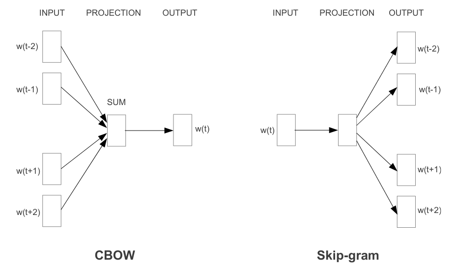
word2vec comes in two flavors, both able to learn word embeddings: CBOW (Continuous bag-of-words) and SG (skip-gram).

wordvec model architectures

word2vec architectures/algorithms

CBOW: Continous bag-of-words

This architecture predicts a word from a window of surrounding context words. This approach looks intuitive. However, Tomas Mikolov, word2vec principal author, says CBOW is less effective when predicts rare words.

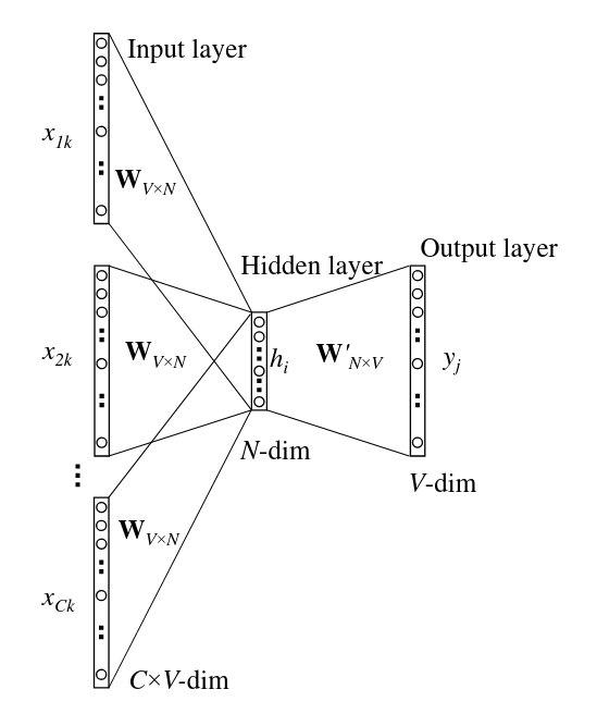
The continuous bag-of-words model

SG: Skip-grams

In this case, the model uses a center word $w_t$ to predict the surrounding window of $m$ context words. SG is less intuitive than CBOW but is a popular selection because of its ability to predict uncommon words better (even with the extra computation cost it requires).

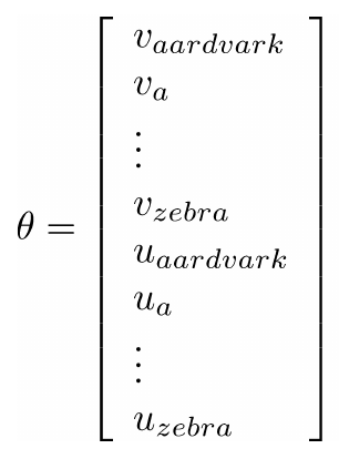
In SG, the vector $\theta$ stores the model parameters. The model's likelihood (probability indicating how good our model is at predicting words around every word) is:

The objective function of the model, $J(\theta)$, is the average negative $log$ of $L(\theta)$ which we want to minimize though SGD (notice that the vector space is enormous):

As with CBOW, the final goal of the model is to obtain word vector representations that embed meaning, but we don't achieve this objective directly. The skip-gram algorithm learns to predict context words given a center word. In this process, and as a by-product, it produces vector representations of words that are good at storing meaning and similarity information.

The skip-gram model

The skip-gram model uses a neural network to output the probability distribution that the word $o$ falls within the contextual window of $c$. This conditional probability can be expressed as $P(O=o|C=c)$ for the given words $o$ and $c$. The expression of this probability is:

We want to optimize SG's objective function, meaning we want to maximize this probability, which has a direct implication on having better word vectors.

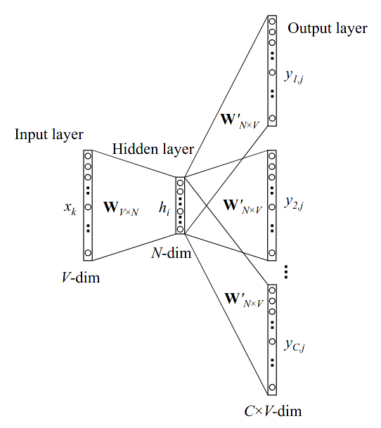
Before exploring the training techniques it is important to extend the architecture description of the skip-gram model. Let's use this excellent diagram by Eric Kim:

The skip-gram model's architecture

The components of this architecture are:

• We use a couple of $N$-dimensional vectors to represent each word. If the word acts as a context word, we represent it as $u_o$. If the word acts as a center word, we represent it as $v_c$.
• Our training corpus is composed of $T$ words and has a vocabulary of $|V|$ words.
• The matrix $U$ (a.k.a. $W_{output}$) contains the "outside" word vectors, meaning, the representation of words when acting as context words.
• The matrix $V$ (a.k.a. $W_{input}$) contains the "center" word vectors, meaning, the representation of the words when acting as center words. When training is over, we use this matrix as our word embeddings.
• During training, we select a context window of size $C$.
• $\hat{y}_{c}$ represents the probabilities of all words in the vocabulary being in the context of the center word $c$.

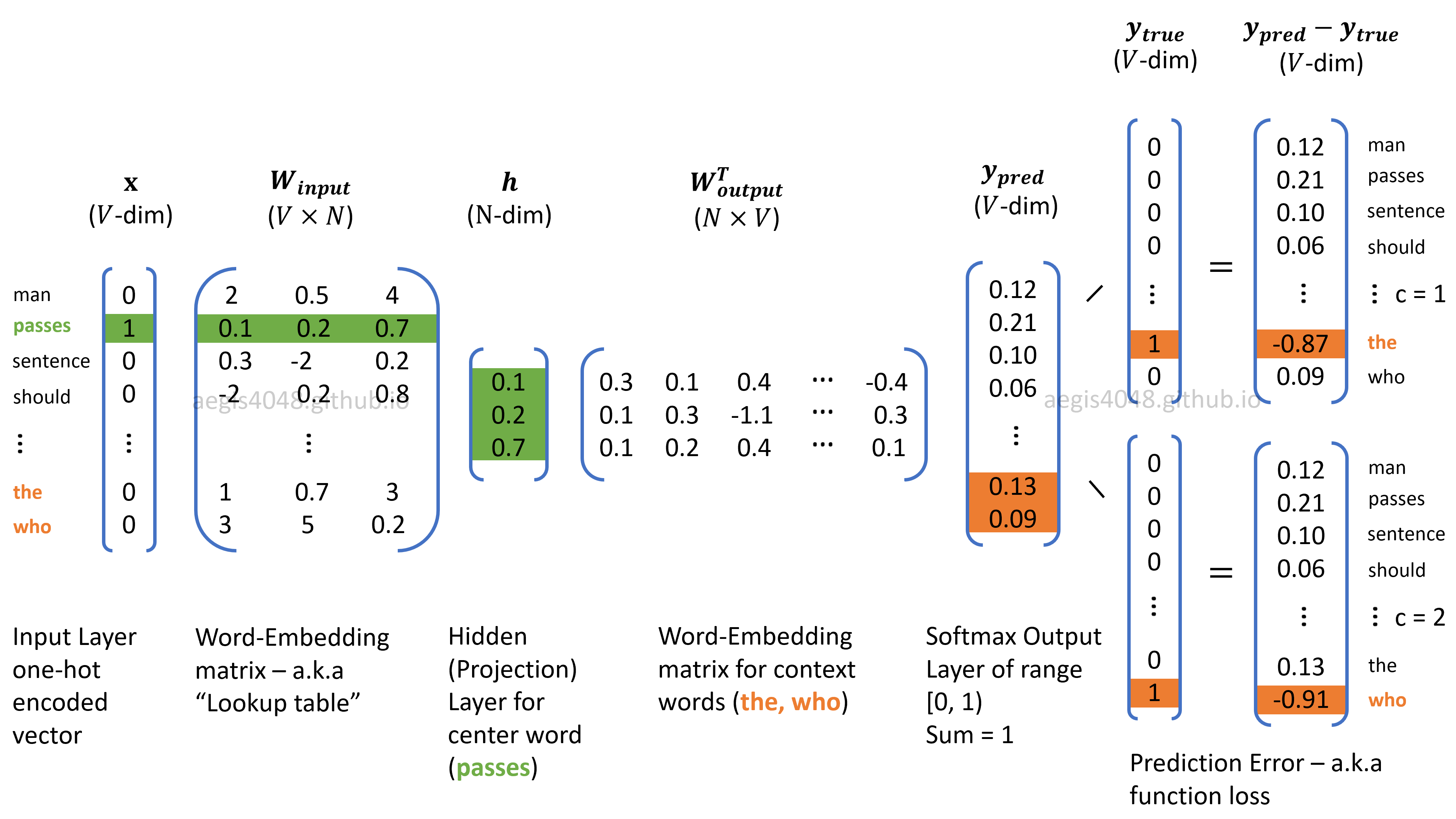
The learning process starting from the left is like this:

• The model receives as input a one-hot vector representing the center word to analyze.
• We use the $V$ matrix to select the corresponding vector $v_c$ given the input the model received.
• We use the $U$ matrix to calculate how similar $v_c$ is to other words in the vocabulary.
• We calculate the prediction error and use it to update the parameters in our $\theta$ vector.
• We move to the next word in the vocabulary and start the process again.

word2vec training techniques

The default training process of word2vec uses the softmax function. As we can see in equation (3), this is expensive in terms of computing time. Fortunately, we can use an alternative method to reduce this complexity.

The alternative methods fall into two groups: Softmax-based and Sampling-based. The most common techniques are Hierarchical Softmax and Negative Sampling. In this article, I'll focus on the latter.

Hierarchical Softmax

It uses a hierarchical binary tree to represent words as leaves. The probability of a word is decomposed into a sequence of probabilities. We start at the root of the tree and take decisions until we reach a leaf-word. The final probability is computed by the path we followed.

Negative Sampling

This technique don't use the Softmax function. It approximates the objective function by sampling $K$ negative examples. Then our objective function is transformed into:

Where:

• $\sigma$ is the sigmoid function
• The negative samples are $w_1, w_2, \dots, w_K$ with outside vectors $u_1, u_2, \dots, u_K$
• The outside word $o \notin \{w_1, w_2, \dots, w_K\}$

As we can see, we got rid off the expensive denominator of the Softmax function!

How can we code this?

We first need to dig deeper into word2vec. The first thing to notice is that the Softmax loss presented in equation (2) is the same as the cross-entropy loss between the predicted and true distributions. The intuition behind this affirmation is:

• The Softmax outputs a distribution where all probability mass is on the correct class.
• "The cross-entropy objective wants the predicted distribution to have all of its mass on the correct answer" (for more information read here).

This equivalence helps us when doing the derivation of the loss function w.r.t. its parameters as we can see below. But what is $\theta$? Simply speaking is the complete vocabulary of the corpus we are using for training. But as we are representing each token with two vectors, then we have a vector in the $\Reals^{2N|V|}$ space. Yeah, this is huge!

Source: CS244N

Note: The code snippets presented below are part of the full implementation of word2vec. You can see it here.

Naive Softmax Derivation

Let's remember that for a single pair of words $c$ and $o$:

Then, and per the cross-entropy equivalance for the same single pair of words, we have that:

$y_o$ is a one-hot vector, so:

Similarly, we can calculate the derivative of $J(\theta)$ w.r.t. $u_w$ considering the cases where $w = o$ and $w \neq o$ :

Here we have to notice that, as we are following the shape convention, the result of $\frac{\partial}{\partial U} J(v_c, o, U)$ should have a shape of $|V| \times N$. That means we should use a cross product instead of a dot product in the gradient calculations.

With these results, the implementation of the softmax loss and gradients is easy. The function to calculate this receives as parameters the current center vector $v_c$, the outside words matrix $U$ and an index of the current context word $u_o$ we are analyzing on this iteration:

def naiveSoftmaxLossAndGradient(
    centerWordVec,
    outsideWordIdx,
    outsideVectors,
    dataset
  ):

    W_oT_dot_v_c = np.dot(outsideVectors, centerWordVec)
    y_pred_vc = softmax(W_oT_dot_v_c)

    y_true_o = np.zeros_like(y_pred_vc)
    y_true_o[outsideWordIdx] = 1

    # Loss for the current v_c and u_o
    loss = -np.log(y_pred_vc[outsideWordIdx])
    pred_error = y_pred_vc - y_true_o

    gradCenterVec = np.dot(pred_error, outsideVectors)  # dJ/dv_c
    gradOutsideVecs = np.outer(pred_error, centerWordVec)  # dJ/dU

    return loss, gradCenterVec, gradOutsideVecs

Negative Sampling Derivation

As we have seen above, it is expensive to calculate the Softmax's gradients and loss for each iteration. We can solve this by considering just a subset of the vocabulary composed of $K$ words as shown in equation (4).

The derivatives of the Negative Sampling loss function look like this:

Notice the need of making the calculations in parts for $u_k$. As we need a for loop to implement this I think it is advisable to take advantage of it to accumulate the values for the loss and the gradient w.r.t. $v_c$:

def negSamplingLossAndGradient(
    centerWordVec,
    outsideWordIdx,
    outsideVectors,
    dataset,
    K=10
  ):

    [...]

    u_o = outsideVectors[outsideWordIdx]
    v_c = centerWordVec
    uovc = np.dot(u_o, v_c)

    gradOutsideVecs = np.zeros_like(outsideVectors)

    # dJ/u_o
    gradOutsideVecs[outsideWordIdx] = np.dot(v_c, sigmoid(uovc) - 1)

    # For the negative samples
    sum_for_loss = 0
    sum_for_dJ_vc = 0

    for k in negSampleWordIndices:
      u_k = outsideVectors[k]
      minusukvc = np.dot(-u_k, v_c)

      # dJ/u_k
      gradOutsideVecs[k] += np.dot(-v_c, sigmoid(minusukvc) - 1)

      # Let's take advantage of the for loop
      sum_for_loss += np.log(sigmoid(minusukvc))
      sum_for_dJ_vc += np.dot(u_k, sigmoid(minusukvc) - 1)

    loss = -np.log(sigmoid(uovc)) - sum_for_loss
    gradCenterVec = np.dot(u_o, sigmoid(uovc) - 1) - sum_for_dJ_vc

    return loss, gradCenterVec, gradOutsideVecs

The skip-gram model

Now the we have the building blocks for the parameters update, we can continue coding word2vec. The next step is adding the skip-gram model for a center word $c = w_t$, and a context window $[w_{t-m}, \dots, w_{t-1}, w_t, w_{t+1}, \dots w_{t+m}]$ where $m$ is the context window size. As we saw in the previous post, the total loss for the context window is:

Observe we can plug the naive Softmax or Negative Sampling loss in the equation. The calculations of the total loss and the gradients for the current center word $v_c$ can be implemented as follow:

def skipgram(currentCenterWord, windowSize, outsideWords, word2Ind,
             centerWordVectors, outsideVectors, dataset,
             word2vecLossAndGradient=naiveSoftmaxLossAndGradient):
    loss = 0.0
    gradCenterVecs = np.zeros(centerWordVectors.shape)
    gradOutsideVectors = np.zeros(outsideVectors.shape)

    vc_idx = word2Ind[currentCenterWord]

    for u_o in outsideWords:
        partial = word2vecLossAndGradient(
            centerWordVectors[vc_idx],
            word2Ind[u_o],  # index of the U matrix for current context word
            outsideVectors,
            dataset
            )

        loss += partial[0]
        gradCenterVecs[vc_idx] += partial[1]  # Update the parameter v_c
        gradOutsideVectors += partial[2]  # Update the parameter U

    return loss, gradCenterVecs, gradOutsideVectors

SGD: Tying it all together

We are now ready to train our model and get our word embeddings with word2vec. How do we do it?

• Load the training corpus
• Define the vector embeddings dimension
• Define the context size
• Initialize the matrices $U$ and $V$ with random values
• Run SGD until convergence. On each iteration execute the skip-gram model for a center word and its context words. Use the returned loss and gradient values to update the parameters

You can check the related code here.

How do the resulting word embeddings look?

We can take a small number of words to display and see how they relate to each other. For example:

visualizeWords = [
    "great", "cool", "brilliant", "wonderful", "well", "amazing",
    "worth", "sweet", "enjoyable", "boring", "bad", "dumb",
    "annoying", "female", "male", "queen", "king", "man", "woman", "rain", "snow",
    "hail", "coffee", "tea"]

The vectors look like this after 40k iterations and 6598 seconds:

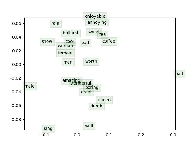
Source: Own. Notice we are losing information when moving from multidimensional space to 2D when representing the vectors in the image.

Now What?

Well, this is just the beginning of the journey! As I said before, word embeddings are a cornerstone for NLP. It is critical to understand it well and, whenever possible, continue learning about it.

This framework is also a fantastic introduction to ML since it presents a basic "neural network" architecture and uses SGD, a fundamental concept for any ML professional.

I'm sure these calculations will later appear as I move forward in my learning path, and I'll need to go deeper and farter: yeah! 🤓. For the moment, it has been a pleasure, and it is time to start checking what can I do with this new toy: the word embeddings!