In the previous post, I reviewed recurrent neural architectures applied to the solution of an everyday problem, translation. And while it is true that the results were quite good (for a testing scenario), there are several reasons why RNNs have lost popularity, and we now live in a world where the Transformer is king.

The main reasons for the disuse of RNNs are:

• Difficulty to learn long-distance dependencies
• Limited time and resources savings due to their sequential nature.

These reasons, plus the recent accessibility to specialized parallel computing cores such as TPUs, have led to the decline of architectures such as LSTMs, GRUs, and other types of RNNs in favor of Transformer-based models.

Due to this popularity, I want to focus this article on Transformer architecture, reviewing it through a simple model capable of predicting a person's birthplace. I also analyze the structure of the training dataset to understand how its dimensions change when doing the Attention calculations.

Finally, I explore the transfer learning paradigm by running several training passes and evaluating their results to see how much pretraining helps us achieve better results.

Table of Contents

• A quick overview of the Transformer architecture

• The multidimensional journey of inputs

• A dimensional-wise closer look to the Encoder's Multi-Headed Self-Attention

• Pretraining, the master key

  • Model $\alpha$: A model to predict the place where a person was born
  • Model $\omega$: Pretraining the model with Wikipedia data
  • Bingo!: Using the $\omega$ parameters to improve the $\alpha$ model

• Are we there yet?

A quick overview of the Transformer architecture

The Transformer Architecture. Source: Dive into Deep Learning

A Transformer is a seq2seq model composed of a stack of encoders that receives an input. These encoders produce an output that feeds a stack of decoders in charge of making predictions. Despite the excellent results Transformers have helped us to achieve, they also come with some drawbacks. The biggest one is the quadratic computation cost present in the Self-Attention mechanism.

If you are new to this kind of architecture, I'd recommend starting with this excellent lecture by professor Pascal Poupart of the University of Waterloo.

After reviewing this architecture, these are the most relevant points I noted:

• The input data ($X$ or Sources in the image above) shape is $(b,n,d)$. Where $b$ is the batch size, $n$ is the input sequence length, and $d$ is the dimension of each item in the input sequence.
• The Encoders stack output has the same shape $(b,n,d)$. The Decoders stack and the Encoder-Decoder Multi-Head Attention unit in the Decoder expect the same tensor shape.
• The Encoder (all layers) runs once per input batch.
• The second Encoder in the stack receives as input the output of the previous Encoder in the stack. This happens across the stack except for the last Encoder, which output feeds the Encoder-Decoder Multi-Head Attention unit in the Decoder.
• The Encoder's Multi-head Attention unit's input (queries, keys, and values) comes from the previous Encoder layer, except for the first Encoder. In that case, they come from the input $X$.
• The Decoder (all layers) runs multiple times. Each time the Decoder outputs a prediction.
• The Decoder's Masked Multi-head Attention unit's input (queries, keys, and values) comes from the previous Decoder layer, except for the first Decoder. In that case, they come from the input $Y$ (Targets).
• The Encoder-Decoder Multi-Head Attention unit receives three parameters:
  • Query: The output of the previous Decoder layer.
  • Key, Value: The Encoders stack's output. These values are also called Memory.
• The FC element in the image represents a Linear Layer followed by a Softmax function to produce a probability distribution to select the Decoder's output.
• The Positionwise FFN applies transformations to the Attention outputs to model complex interactions of the sequences.

What about the information received by the Encoder? How is the transformer fed?

The multidimensional journey of inputs

I have always thought that we can learn a lot from a system if we pay attention to the data flowing across the system's components. Perhaps this kind of analysis is part of the interpretability efforts to describe what NN are doing, undoubtedly, an interesting topic I hope to explore in the future.

In this case, I examined the pathway and transformations the dataset experience within a character-level model. This model is a fork of Andrej Karpathy's minGPT, with modifications done by Stanford's CS224N TAs (thank you guys!). You can find the complete codebase here. The objective of the model is to predict the place where a person was born.

To improve the model's performance, we first executed a pretraining phase to build knowledge about a person's name and its place of birth. The image below shows a simplified view of the training modules and how the data moves between them:

Source: Own

As the image shows, the train_dataset variable stores the training dataset. This variable is an object containing sentences with person names and the places where they were born, for example:

Eyolf Kleven. Born in Copenhagen, Kleven played as a midfielder for AB from 1927 to 1944 .

We'll later use these sentences to apply a span-corruption algorithm that will be the base of the pretraining objective. The sentences are transformed into numeric values by using a simple mapping against the dataset vocabulary. As our sequences are made of characters, the above example now looks like this:

tensor([33, 80, 70, 67, 61,  3, 39, 67, 60, 77, 60, 69, 14,  3, 30, 70, 73, 69,
         3, 64, 69,  3, 31,  1, 60, 69,  3, 71, 67, 56, 80, 60, 59,  3, 56, 74,
         3, 56,  3, 68, 64, 59, 61, 64, 60, 67, 59, 60,  1, 70, 71, 60, 69, 63,
        56, 62, 60, 69, 12,  3, 39, 67, 60, 77,  0,  0,  0,  0,  0,  0,  0,  0,
         0,  0,  0,  0,  0,  0,  0,  0,  0,  0,  0,  0,  0,  0,  0,  0,  0,  0,
         0,  0,  0,  0,  0,  0,  0,  0,  0,  0,  0,  0,  0,  0,  0,  0,  0,  0,
         0,  0,  0,  0,  0,  0,  0,  0,  0,  0,  0,  0,  0,  0,  0,  0,  0,  0,
         0])

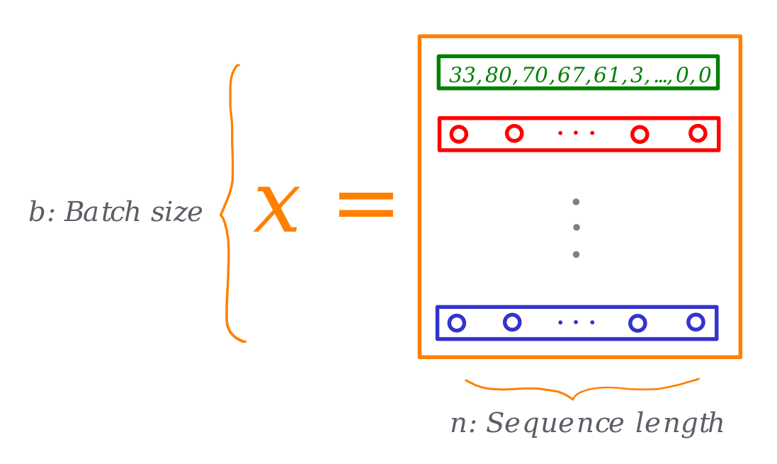
The number 0 represents the pad token we use to ensure all sentences are equal in length, the number 1 represents the span-corruption character. And the first number, 33, represents the letter E from "Eyolf".

At this point (up until GPT.forward) the batch of training examples we are feeding into our transformer looks like this:

Source: Own

As these fixed representations of characters don't allow learning the existing relationships between them, we need to add a new dimension. We do this in the forward pass of the Transformer blocks:

def forward(self, idx, targets=None):
    b, t = idx.size()
    assert t <= self.block_size, "Cannot forward, model block size is exhausted."

    # forward the GPT model
    token_embeddings = self.tok_emb(idx) # each index maps to a (learnable) vector
    position_embeddings = self.pos_emb[:, :t, :] # each position maps to a (learnable) vector
    x = self.drop(token_embeddings + position_embeddings)
    x = self.blocks(x)
    x = self.ln_f(x)
    logits = self.head(x)

    # if we are given some desired targets also calculate the loss
    loss = None
    if targets is not None:
        loss = F.cross_entropy(logits.view(-1, logits.size(-1)), targets.view(-1), ignore_index=0)

    return logits, loss

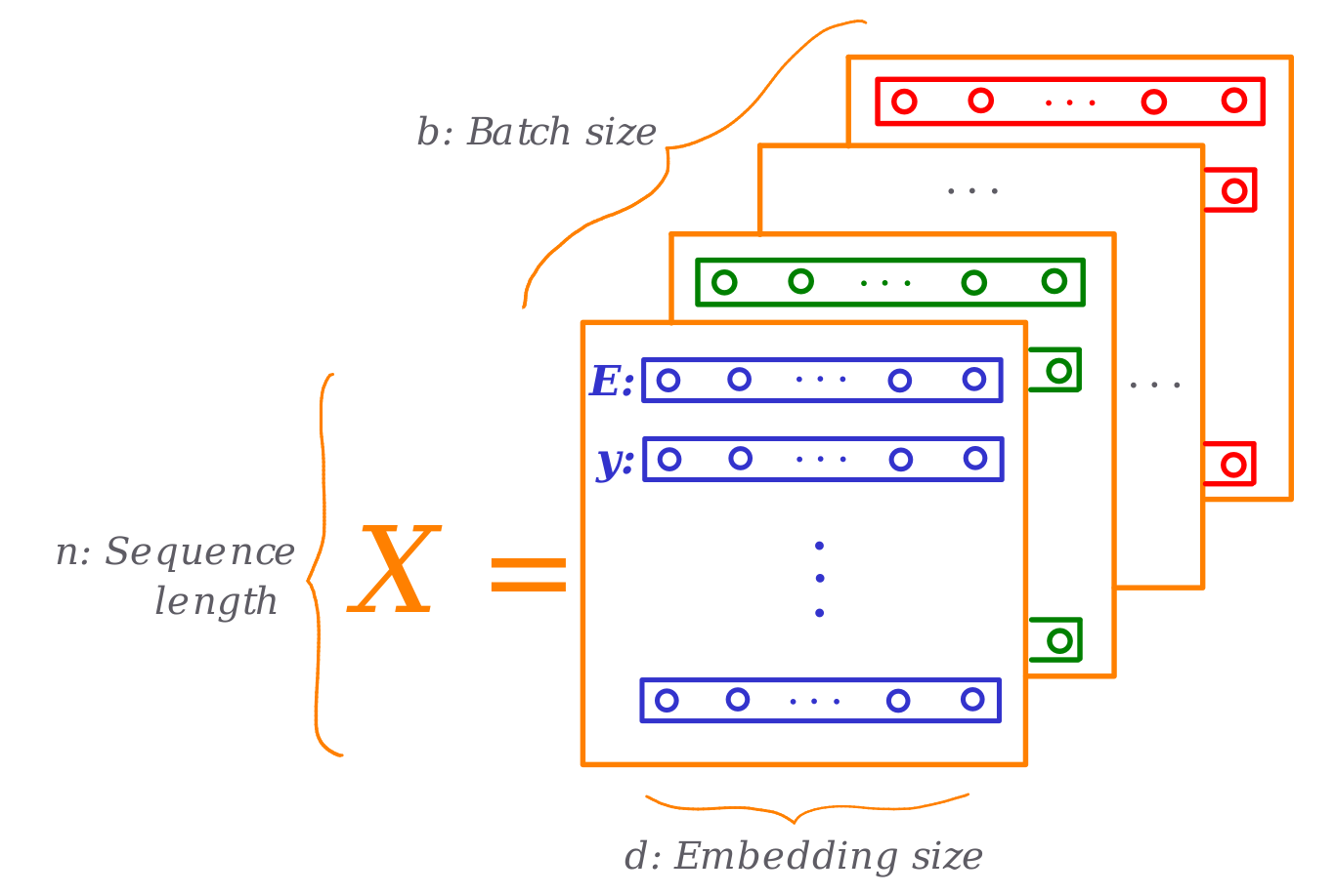
As you can see, we add the token and position embeddings to the input we received from the run_epoch loop. Our input data structure now looks like this:

Source: Own

Notice how each letter (integer number) is now represented with a $d$-dimensional learnable vector. From now on, this input representation ($X_{b, n, d}$ in the following paragraphs) is used through the model calculations. For example, the Attention mechanism will use these vectors to draw the queries, keys, and values to compare against other parts of the input space.

A dimensional-wise closer look to the Encoder's Multi-Headed Self-Attention

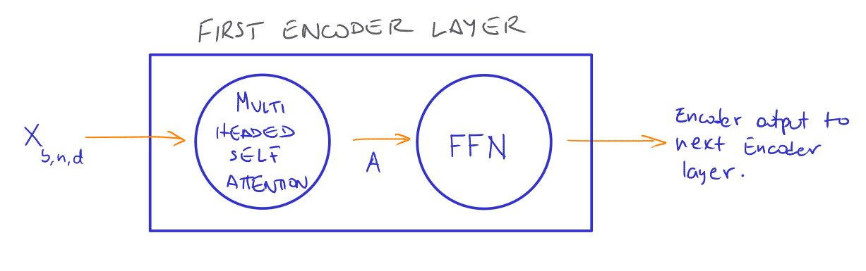
Now, how does the Multi-Head Attention calculation takes place within the Encoder? To answer this question, it is needed to determine how the tensors and weight matrices interact through the network. If we remember, any Encoder layer contains two sub-modules, the Multi-Headed Self-Attention mechanism and an FFN:

Source: Own

Where $A$ is the $Atttention$ output and is calculated like this:

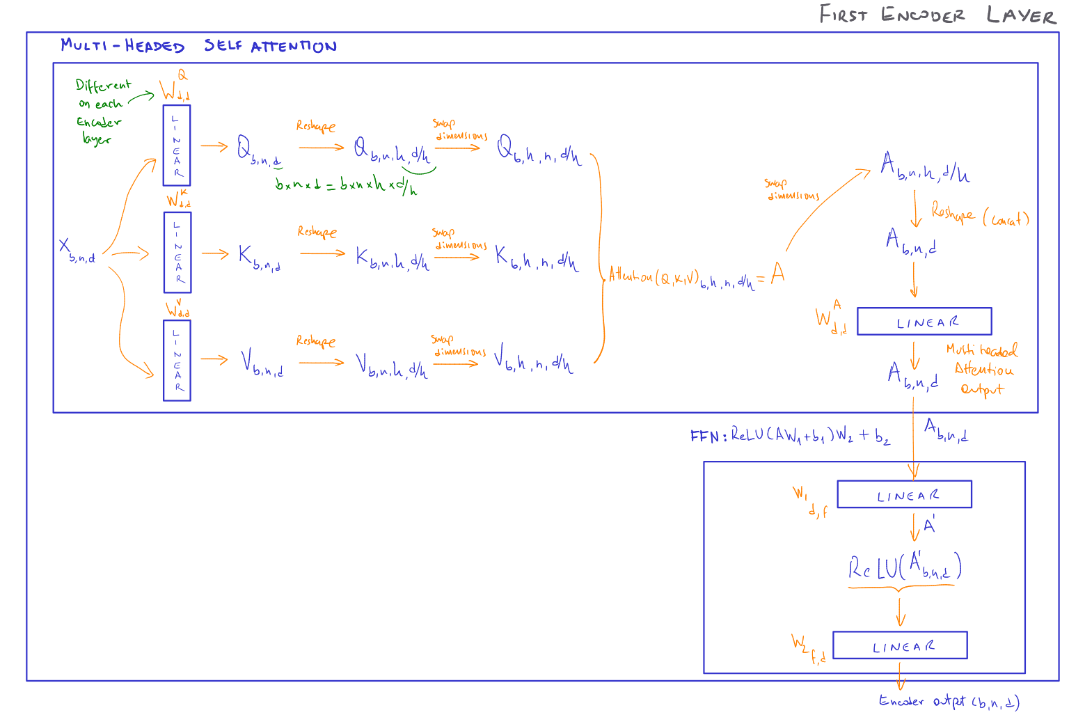
Let's take a closer look at the Attention mechanism (in this case based on a scaled dot-product scoring function):

Source: Own

As we can see in the image, the input tensor $X$ acts as query, key, and value. We can obtain and learn these parameters by applying the three linear transformations shown earlier.

Dimension-wise, as $X$'s shape is $(b, n, d)$, the output of the linear transformations will keep the same size. As we want to learn the interactions between different parts of $X$ and identify which elements are more relevant than others, we split the input tensor into $d/h$ chunks, where $h$ is the number of Attention heads to use. Each head will focus on a particular aspect of the input, meaning the Attention calculations happen head-wise. To allow this, we reshape the tensors into $(b, h, n, d/h)$ where the second and third dimensions are swapped to allow matrix operations.

As we are using a dot-product scoring function, we need to interchange the dimensions of the $K$ tensor into $(b, h, d/h, n)$ before multiplying it with the $Q$ tensor. This product will produce a tensor of shape $(b, h, n, n)$.

To get the Attention output, we apply the Softmax function and multiply the results with the Values tensor $V$ getting an Attention output tensor of shape $(b, h, n, d/h)$.

In this last tensor, we have the Attention calculations for all heads, we concatenate them together by reshaping the tensor into $(b, n, d)$ using the view method. As we can notice, the last tensor, the Attention output, can now be fed into the FNN, which will produce a tensor of the same shape. The resulting tensor is the Encoder output, which will serve as input of the next Encoder layer, or, if it was the last Encoder, as input to the Encoder-Decoder Multi-Head Attention mechanism of the Decoder.

Pretraining, the master key

Initially, we run a supervised training of our model with a small dataset to teach it to predict the birthplace of some people, but the results were not precisely good :)

How can we improve this? Of course, we can increase the training dataset size, but we can also initialize our model parameters differently. That is the idea behind pretraining. Pretraining trains our model in two steps:

• Unsupervised train our model to learn statistical properties of the language like syntax, semantic, sentiment, and other types of relationships.
• Retrain our model to perform a downstream task (predicting the birthplace in our case) using the parameters from the previous step.

The second step, also know as Finetuning, is supervised training for our downstream task. This technique is an excellent idea since the parameters learned in the first step include some general knowledge about the language, making the second training step quicker, more effective since it requires less data.

This new paradigm comes in three flavors, all of them using the Transformer architecture:

1. Pretraining using a Transformer Decoder. This modality has had enormous success in language generation. For example, the GPT models by OpenAI, which last version, GPT3, has 175 billion parameters. This model has generated a lot of hype lately for its capacity of generating human-like text.

   
   A GPT-3 generated news article. Source: Language Models are Few-Shot Learners

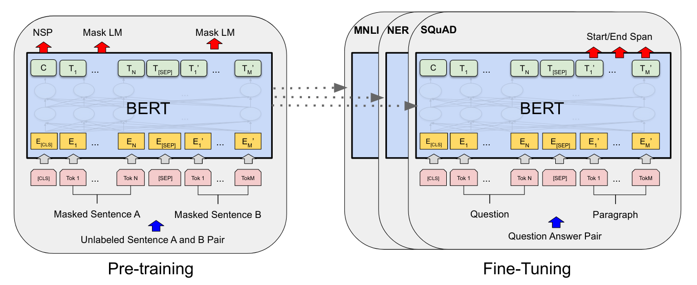
2. Pretraining using a Transformer Encoder. This modality is also popular and successful. For example, in 2019, Google started to use the BERT model to process its search engine queries.

   
   Overall pre-training and fine-tuning procedures for BERT. Source: BERT: Pre-training of Deep Bidirectional Transformers for Language Understanding

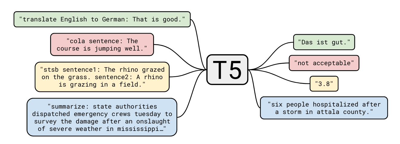
3. Pretraining using a Transformer Encoder and Decoder. Here we have the T5 model. The paper describing this model includes multiple configurations and combinations of hyperparameters that allowed the authors achieve SOTA results in various downstream tasks through finetuning.

   
   A diagram of T5 text-to-text framework. Source: Exploring the Limits of Transfer Learning with a Unified Text-to-Text Transformer

So it seems this is the way to go these days: pre-train your model and then use its parameters to initialize the model's parameters for the second round of training (finetuning) using a downstream objective and dataset.

Let's see this paradigm in action in the next section. Each training task (except the finetuning) was done in about 2 hours using an Azure GPU VM with the following characteristics:

• 6 vCPUs with 56GiB RAM
• 1 NVIDIA Tesla K80 GPU with 12GiB RAM
• 150 GiB of SSD storage
• Linux Ubuntu 18.04

Model $\alpha$: A model to predict the place where a person was born

We feed the model with a dataset containing a question about the place of birth of a person and then the ground truth. Something like this:

Where was Eyolf Kleven born?	Copenhagen
Where was Marvano born?	Belgium
Where was Naïma Azough born?	Morocco
Where was Eugenia Popa born?	Bucharest

The configuration was:

• A Transformer with 4 Encoder/Decoder layers
• 8 Self/Attention heads
• 256-dimensional embeddings
• 75 epochs
• Batch size of 256
• LR of 6e-4

The performance after training was not good, compared with the baseline of predicting "London" for any input question (correct rate of 5%). This result is not surprising, considering that the training dataset size is small. Either way, it is fine since the purpose of the exercise is not to achieve top results but to see how pretraining boosts the model's performance.

Model $\omega$: Pretraining the model with Wikipedia data

How to improve the performance of our model? One evident option is to increase the size of our supervised training dataset. Sadly, it might not be viable since the cost of creating a large custom dataset can be prohibitive. Also, increasing the dataset size will increase the computation cost due to the Attention quadratic nature.

A solution for this case is pretraining. In this example, we are using a larger unsupervised dataset from Wikipedia. The dataset contains the name of a person and the corresponding birthplace. Regards the training objective, we set it to predicting a corrupted span of the input sequence.

The input entries look like this:

Greta Knutson. Born in Stockholm, Greta Knutson studied at the Kungliga Konsthögskolan, and settled in Paris, France during the early 1920s .
Paul Daniels. Paul Daniels (born 4 June 1981 in Burlington) is an American rower .
Tom Jones. Tom Jones (born April 26, 1943) is an American former racing driver, born in Dallas, Texas .
Elizabeth Bartlett. Elizabeth Bartlett (24 April 1924 Deal, Kent - 18 June 2008) was a British poet .

The training settings were these:

• 4 Encoder/Decoder layers
• 8 Self/Attention heads
• 256-dimensional embeddings
• 650 epochs
• Batch size of 128
• LR of 6e-3

After training, we saved the model parameters on disk for later use.

Bingo!: Using the $\omega$ parameters to improve the $\alpha$ model

Now it is time to check if pretraining helps. To do it, we loaded the parameters from the pretraining stage and retrain the model with the downstream task dataset (question/answer pairs). The training parameters were as follow:

• 4 Encoder/Decoder layers
• 8 Self/Attention heads
• 256-dimensional embeddings
• 10 epochs
• Batch size of 256
• LR of 6e-4

The model's evaluation showed that the performance increased 14 times! Wow!, that is amazing, considering we just run the finetuning task for ten epochs.

These results are a confirmation that the combo pretraining + finetuning + Transformer architecture is the holy grail of Machine Learning since 2017. It just works.

Are we there yet?

While it is true that the Transformer is crucial to achieving SOTA results in various NLP tasks, they are not perfect. Recent AI's community efforts center on reducing or even eliminating the quadratic operations in the Attention mechanism.

During this exercise, we also implemented an alternative Attention computation that eliminates the quadratic cost. It was a variant of the Synthesizer Attention for the pretraining and finetuning tasks. Unfortunately, the results were not promising (similar to the baseline, of course, this is better than the Model $\alpha$ performance, but still modest).

What now? I am finally concluding my journey of learning modern NLP. It is satisfying and exciting to review more and more recent papers. I now feel much better prepared to face the upcoming challenges in my career. It is time to continue reading about the Attention mechanism and its improvements and how to apply this architecture to solving everyday problems for personal or business use cases!

As Dr. Károly Zsolnai-Fehér says: "What a time to be alive!"



👋