Implementing a Transformer-based Translator with Tensorflow 2.6 and Google Cloud ⛅
Impressions from coding locally and deploying/training remotely
At some point, it becomes tedious to work with Kaggle or Colab, and you need to have more flexibility to produce better code. In this article, I detail key challenges of remote training, delve into crucial Transformer concepts, and share some practical tips for accomplishing this task.
I am now accumulating practical experience building end-to-end NLP models and deploying them in production environments to attend other services through APIs. Until now, I had programmed and trained models locally on my laptop or in virtual environments like Kaggle or Colab, but I have seen these environments have limitations that make it difficult to keep making progress.
Thanks to my latest experiences, I feel I have moved up one more level in my NLP path, and now I am more comfortable working under a scheme analogous to what I might find in a company. And although I don't know any Machine Learning Engineers to ask, I imagine their way of working is similar to the following:
They probably use laptops instead of desktop computers.
The laptops probably have an NVIDIA GPU.
These laptops should be sufficient to train a small model but not enough to train giant models like GPT3.
Large models training happens on remote VMs, so they have subscriptions on GCP, AWS, or Azure.
Engineers code locally and deploy to VMs in the cloud. They presumably debug the code remotely from their local IDE.
They use tools like TMUX in the VMs to start training from their laptops.
I consider it crucial for me to have an experience like the one I have described, and in pursuing it, I came across interesting situations that I want to share in case it helps someone on a similar path to mine.
This article also talks about the new things I have learned from working with a Transformer.
Kaggle works great for learning or doing experiments. But if you need a recent TensorFlow (TF) feature, it is likely not getting it easy. Kaggle's TF default version is 2.4.1. You can update it with !pip install --upgrade tensorflow, but when you stop the session and start it again, the new instance will have TF 2.4.1. The same happens with additional packages not included in the Docker image used to create Kaggle's VMs. As I want to use some features present since version 2.5.0, I discarded this platform.
Colab's default VMs come with TF 2.6.0. But as with Kaggle, their VMs are ephemeral, and new packages will be lost when restarting them. Also, Colab lacks the script view, meaning it is conceived to be used with interactive notebooks. Perhaps it is possible to use your Google Drive to store your modules and import them from there, but I haven't tried that yet. Still, it is a nuisance to grant Colab permission each time you start a new session. Besides these limitations, the worst one, for me, is that if you run a model on Colab for several hours, you will be temporally banned as they prefer interactive usage of their hardware and disfavor long training with their GPUs.
Don't get me wrong, I love both platforms, but I guess their use cases are different from what I need right now.
There are obscure workarounds for some issues I mentioned earlier, like mounting your Google Drive and install the packages there, but I find that too messy since you'll need to update the Python paths, something I prefer to avoid.
If not them, who?
My need is not "free GPU" but an entire work environment for Machine Learning. I thought of Sagemaker, but it seems the trial period doesn't include GPU instances. Anyway, I thought it would be better to choose another provider since I already had some exposure to AWS.
I researched a little bit and tried some products like Datalore, Deepnote, and Paperspace. But for pricing, trial limitations, or functionality, I discard them for the moment.
Once you have started a trial period, the first thing you have to do is to switch to the entire GCP experience. Meaning, you have to add your credit card details. It is OK, you still have the free credits for three months, and you can use them before charging anything to your card.
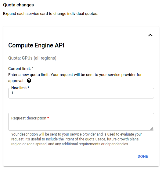
Next, you have to ask for a global GPU quota increase. It is needed because the trial period doesn't include GPU usage.
Source: GCP
Now we are ready to create a VM. There are several ways to do it. The easiest one I found was to create a new notebook on GCP's AI Platform. It allows you to customize its characteristics and includes all drivers and settings needed for the GPU to work out of the box with TF. Once the VM instantiates, you can log in remotely with SSH from your laptop.
There is an intricate way to work with Colab's VMs locally and without notebooks. But it is complex (exposes a public IP through ngrok), and given Colab's limitations, I think this option doesn't deserve the effort.
Setting up the local environment
I prefer to work with an IDE. I tried the Spyder IDE, looks great, but I couldn't make it work with Poetry, my defacto dependency manager. I also thought on Emacs, but I didn't want to dedicate much time to set it up for this (I like you Emacs, but you are high-maintenance, not now, sorry :). The most obvious options for me would be VSCodium or PyCharm. Both can work with remote interpreters (BTW, the path to the base Conda env. is ~/opt/conda/bin/python3) and are good choices if you want to use a lightweight computer for ML.
The setup for enabling remote deployment is well documented online. It is easy once your VM has registered your public key. The only annoying thing is that you need to update your SSH/deployment profiles each time you start your VM instance since it grabs a different IP address. But in the long term, it is nice to have persistent storage, a good amount of RAM, and a dedicated GPU for your experiments.
Do not forget to stop your VM instance when you finish using it. Otherwise, it might consume all your credits and even incur charges to your credit card!
Coding a Transformer
Conda or not Conda?
One of the things I dislike the most is bloating. In general, I try to avoid a VM with a default Conda installation. I admit it is practical because it provides a complete working environment with all the libraries and frameworks you might need, but most of the time (my experience), you won't ever use them all. I prefer a zen approach, like an empty VM where I could add the packages I need with Poetry without unnecessary dependencies filling up the disk for nothing.
In this case, as I didn't want to spend time on the CUDA configuration, I chose a pre-configured VM with Conda.
In general, my recommendation would be to use Conda if you don't want to worry about missing dependencies or issues with the GPU support. If needed, you can remove packages manually to lighten your VM. Optionally, you can create a new Conda environment, but be careful with Conda's folder permissions. The owner will probably be the root user.
Requirements
Since TensorFlow (TF) seems popular in business configurations, it made sense to use it as a framework for coding the translator. It is straightforward and intuitive to use, and its ecosystem contains almost all you'll need to code, train, and deploy any modern ML model.
Now, what version of TF to choose? For general use, I'd say to start with anything above 2.4. In this case, I wanted to build a BERT vocabulary from a dataset. There is a method available for that since version 2.5.0. That method is inside TensorFlow Text. The version of TF Text must coincide with the one from TF. As my VM came with TF 2.6.0, I added TensorFlow Text 2.6.0 using pip (TF Text is not available in Conda yet).
Besides this, I wanted to use the parallel corpora from TensorFlow Datasets, so I added the latest version.
Finally, prompt-toolkit is needed to enable the TUI.
Data as a common thread
I have written about Transformer architecture in the past, and material about it is abundant on the Web. So this time, I'm going to comment on the journey that data takes through the Transformer components and thereby get a different view of how it works.
Working the dataset out
As with everything in ML, it all starts with the data. Which training corpus to use?
TensorFlow Datasets provides several ready-to-use datasets. It is an easy and fast way to start using them for our ML projects. I checked the options for Spanish-English translation, and I came up with a perfect combination for my expectations: The OPUS parallel corpora. It contains humongous corpora of parallel training examples. Much of it comes from government entities like the European Union. I wanted to have a mix of formal and informal examples, so it occurred to me that it would be a good idea to merge the Books and the OpenSubtitles datasets.
In the end, I discovered that only the OpenSubtitles dataset is part of TensorFlow Datasets as of September 2021. I trained the model with it.
EDA?
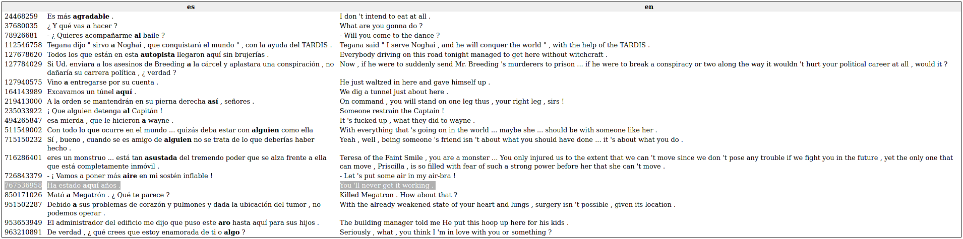
I don't think it is necessary, but at least we should look into the data. In practice, the OpenSubtitles corpora didn't result in the best choice. Mainly because of the particularities of the subtitling job. The examples are short, and a phrase might be translated in different ways by different people. Also, the subtitles are written by amateurs, and some translations are not accurate (some are completely wrong, see image below). Anyway, as this is not a professional setting, I'm OK with these limitations.
Source: Nordic Language Processing Laboratory
Download the dataset once, reuse it many times
The Spanish-English parallel corpus from OpenSubtitles 2018 weighs 1.8G. It contains 500K sentences and 3.1 million English tokens. The idea is to download it once and use a fraction of it to train our vanilla model.
The tfds.builder function helps us with this. It expects a dataset name and download configuration.
This is how the dataset configuration looks like:
  build_config = tfds.translate.opus.OpusConfig(
      version=tfds.core.Version("0.1.0"),
      language_pair=("es", "en"),
      subsets=["OpenSubtitles"]
  )
  # OPUS only provides one split: "train"
  builder = tfds.builder("opus", config=build_config)
In the download configuration we can specify how much training examples to prepare:
  dwn_config = tfds.download.DownloadConfig(
      extract_dir=dwn_path,  # store extracted files here
      download_mode=tfds.GenerateMode.REUSE_CACHE_IF_EXISTS,  # Reuse downloads, fresh dataset
      max_examples_per_split=num_items  # "train" split only
  )
Then we proceed to download and prepare the dataset:
  builder.download_and_prepare(
      download_dir=dwn_path,  # Use the files from here instead downloading again
      download_config=dwn_config
  )
The entire process happens in three steps:
The dataset is downloaded to your computer or VM in the path stored in the download_dir parameter. The default location depends on your configuration. In my VM, it downloaded it into ~/tensorflow_datasets/downloads.
The dataset is extracted into the path stored in the extract_dir parameter.
TensorFlow Datasets prepare the dataset according to the specifications in the download configuration. Once completed, it saves the prepared dataset in the default TensorFlow Datasets folder (in my case ~/tensorflow_datasets/opus/en-es for OpenSubtitles/0.1.0). The opus-train.tfrecord-00000-of-00001 file contains the exact number of training examples specified in the download configuration (max_examples_per_split parameter).
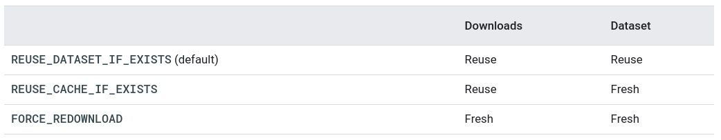
The download_mode parameter defines if it should download/prepare the dataset each time we execute the code. See the summary of this behavior in the following table:
Source: Google
Sadly, it seems the REUSE_CACHE_IF_EXISTS flag has not yet been implemented as of September 2021, so you need to delete the entire opus folder each time you change the value of max_examples_per_split.
About tokenization and vectorization
Ok, we now have downloaded and prepared the training examples. Nevertheless, we can't train a model with the dataset as it is. We need to split the sentences into smaller units and translate those units (tokens) to number equivalences. These processes are called tokenization (sub-word tokenization in this example) and vectorization.
The vectorization translates each subword token into a number. We use each token's index in the vocabularies as a representation.
The tokenization/vectorization of this model uses the BERT tokenizer. The tokenizer requires a vocabulary for each language made from our dataset with the WordPiece algorithm.
We do the entire process in two steps:
Build the vocabulary with the bert_vocab_from_dataset method from tensorflow_text.tools.wordpiece_vocab. As stated by Google, this is a simple implementation. We can found an efficient and scalable implementation (Apache Beam) here.
bert_tokenizer_params = dict(lower_case=True) # Otherwise Que != que
bert_vocab_maker_args = dict(
vocab_size=self.vocab_size,
reserved_tokens=reserved_tokens,
bert_tokenizer_params=bert_tokenizer_params,
learn_params={}
)
en_trn_ds = raw_trn_ds.map(lambda x: x["en"])
es_trn_ds = raw_trn_ds.map(lambda x: x["es"])
es_vocab = bert_vocab_maker.bert_vocab_from_dataset(es_trn_ds.batch(1000).prefetch(2),
**bert_vocab_maker_args)
en_vocab = bert_vocab_maker.bert_vocab_from_dataset(en_trn_ds.batch(1000).prefetch(2),
**bert_vocab_maker_args)
withopen(f"{self.vocab_path}/es_vocab.txt", "w") as file:
file.writelines("%s\n" % token for token in es_vocab)
withopen(f"{self.vocab_path}/en_vocab.txt", "w") as file:
file.writelines("%s\n" % token for token in en_vocab)
As stated in the bert_tokenizer_params, we apply a preprocessing step to the dataset. This procedure transforms the examples by lowering its case, applies NFD normalization, and strips accented characters. As vocabulary creation is an expensive process, it is recommended to do it once and then save the vocabulary files on disk. We will read the files later when tokenizing the datasets.
Construct a custom tokenizer (EnEsTokenizer class) based on the BERT tokenizer provided by TF (BertTokenizer). We use this class to instantiate the tokenizers for both languages using the vocabulary files generated in the previous step.
We are now ready to consume the training dataset by batches of examples, each made of numeric tensors. Let's use them with the following custom training loop:
for (batch, (inp, tar)) inenumerate(train_batches):
_train_step(inp, tar)
if batch % 50 == 0:
print(
f'Epoch {epoch + 1} Batch {batch} Loss {self.train_loss.result():.4f} 'f'Accuracy {self.train_accuracy.result():.4f}'
)
Where:
inp: Are the tokenized Spanish sentences with shape (b,ninp). b is the batch size, and ninp is the length of source examples. It is important to mention that all examples are padded with zeros up to the longest sentence in the batch.
tar: Are the tokenized English sentences with shape (b,ntar). These examples are also padded with zeros up to the longest sentence in the batch.
The training dataset contains train_batches = (train_examples/batch_size).
If we take a look to any of these examples they are like this:
The first item corresponds to the index of the [START] token in the vocabularies. The last item, before the zeros, is the index of the [END] token. If we show the actual tokens we can read the sentence:
These batches are used by the Transformer to predict the next word in the target language (predictions variable):
def_train_step(inp_batch: Any, tar_batch: Any) -> None:
tar_inp = tar_batch[:, :-1] # Decoder's input. We don't need the [END] tokens here
tar_real = tar_batch[:, 1:] # Used to force teach and to calculate loss in predictionwith tf.GradientTape() as tape:
predictions, _ = transformer([inp_batch, tar_inp], training=True) # inp -> Encoder, tar -> Decoder
loss = loss_function(tar_real, predictions)
# Calculate the gradients of the loss function w.r.t. its weights
gradients = tape.gradient(target=loss, sources=transformer.trainable_variables)
optimizer.apply_gradients(zip(gradients, transformer.trainable_variables))
# Store the values
self.train_loss(loss) # Avg. loss of current batch
self.train_accuracy(accuracy_function(tar_real, predictions)) # Avg. accuracy of current batch
The first two lines of the function split the target batch in two:
tar_real is the same as tar, but each of the examples has lost the first token. If we forget of the batches for the moment, and think about the example above, this will be: i wonder if it's bad to be weak [END].
tar_inp is the same as tar, but each one of the examples has lost the last token. Then we have: [START] i wonder if it's bad to be weak. The Decoder uses this element during training. In the first training step, thanks to the look-ahead mask, the Decoder will only see [START] from tar_inp. Then, it should predict the first token in tar_real which is i. The last token in tar_inp (weak) should be used to predict the last token in inp_real which is [END]. This is the reason why we don't need to have the [END] token at the end of tar_inp.
What happens with this data inside the Transformer? Let's see it in the next section.
Going deep into the Transformer
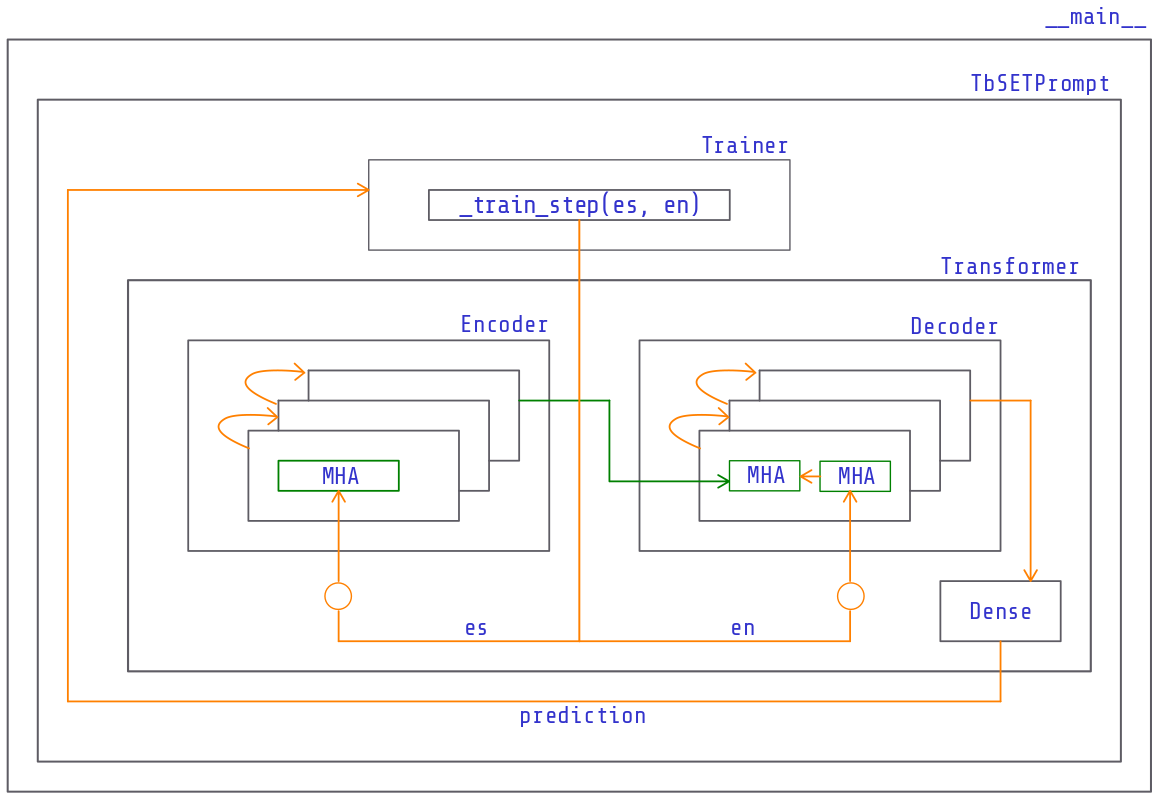
How does the Transformer return a prediction? See the data flow through the architecture in the following diagram:
Source: Own
Within the custom training loop, each training step will:
Invoke the transformer model to generate predictions for the current data batch
Use the predictions to calculate the loss w.r.t. the ground truths (tar_real)
Calculate the gradients using the loss from the previous step
Update the model parameters with the gradients from the previous step
Store the batch loss and accuracy for reporting
The training step is controlled by a GradientTape. It is a TF context manager to record operations for automatic differentiation. In other words, it calculates gradients for later updates with the optimizer:
# Calculate the gradients of the loss function w.r.t. its weights
gradients = tape.gradient(target=loss, sources=transformer.trainable_variables)
optimizer.apply_gradients(zip(gradients, transformer.trainable_variables))
From the TF documentation:
Trainable variables (i.e. created by tf.Variable), including those accessed inside the context, are automatically watched. All resources (gradients) stored in the tape are released as soon as the gradient() method is called unless the persistent=True parameter has been passed when defining the context manager. Only tensors with real or complex dtypes are differentiable.
Let's go into more detail. Each call to the Transformer object will calculate the prediction as follow:
Create the padding and look-ahead masks for the current source and target languages training batches.
Calculate the Encoder's output for the current source language training batch.
Calculate the Decoder's output from the current target language training batch and Encoder's output.
Return as a prediction the output of the Dense layer after the Decoder's output.
Data transformation in Encoder/Decoder before applying Attention
Both components receive numeric tensors representing the source/target word pieces from the original sentences. We don't use these tensors as-is for the Attention calculations. They first go through a sequence of transformations (represented as circles in the diagram above) that include:
Create embeddings for the source/target batches of tensors. More details about this are here.
Add a regularization technique, in this case, a Dropout layer.
After the transformations, we are ready to start the Attention calculations.
Encoding the source batch
The Encoder is composed of a stack of EncoderLayer objects. These layers perform the Multi-Headed Attention (MHA) calculations for the current input batch and pass its output to the following layer:
WiQ,WiK,WiV are parameters matrices acting as projections:
WiQ,WiK∈Rdmodel×dk
WiV∈Rdmodel×dv
WO∈Rhdv×dmodel
dmodel is the source and target embeddings dimensionality.
dk=dv=dmodel/h, where h is the number of heads.
def_scaled_dot_product_attention(q: Any, k: Any, v: Any, mask: Any) -> tuple:# First, calculate QK^T
matmul_qk = tf.matmul(q, k, transpose_b=True) # (b, h, n_q, n_k)# Scale the previous calculation. d_k (depth of k) comes from k:(b, h, n_k, d_k=depth_k=d//h)
dk = tf.cast(tf.shape(k)[-1], tf.float32)
scaled_attention_logits = matmul_qk / tf.math.sqrt(dk) # (b, h, n_q, n_k) sqrt needed to have stable gradientsif mask isnotNone:
scaled_attention_logits += (mask * -1e9)
# Softmax is normalized on the last axis (n_k) so that the scores add up to 1.
attention_weights = tf.nn.softmax(scaled_attention_logits, axis=-1) # (b, h, n_q, n_k)# Multiply with V to get the output
output = tf.matmul(attention_weights, v) # (b, h, n_q, d_v//h)return output, attention_weights
The parameter mask can be a padding or look-ahead mask. The look-ahead mask is used in the Decoder to only attend previous/current tokens when making predictions. Both masks use 1 for values we don't want to consider like the PAD tokens or the "future" tokens. Notice how applying Softmax to the scaled_attention_logits after the += (mask * -1e9) operation will zero out the −inf cells.
For more information about the Attention dimensions during the calculation you can read here.
Decoding the target batch and Encoder's output
The Decoder is composed of a stack of DecoderLayer objects. These layers have three subblocks:
The first one attends the current target language training batch or the output of the previous Decoder layer.
The second one attends the output of the first subblock plus the output of the Encoder's last layer.
The third one is an FFN that processes the output of the second subblock.
With the prediction, we can calculate the loss by comparing it with the ground truth. With the loss, we can calculate the gradients and update the model parameters.
Showtime!
I trained the model for 400 epochs with 114k examples. The final epoch returned a loss of 1.1077 and an accuracy of 0.7303. The time to train one epoch was around 76 secs. The training finished in almost 9 hours with a single Tesla T4 GPU and four vCPUs with 15 GB memory. The cost of the training was about $5. Not bad, eh? :)
The translator at inference time. Source: Own
As a reference, the original Transformer paper trained its biggest model using 8 NVIDIA P100 GPUs during three and a half days.
You can check the complete code for the translator implemented in this article here.
Closing thoughts
I am happy to have done this practical exercise. It took longer than I expected, and the results were not perfect, but that's okay. My goal was not to implement a SOTA model but to learn. There are many things I left undone that are in the next section. No doubt they are relevant improvements, and I hope to do them in the future. Now it is time to continue with adventures in other NLP applications. I am very interested in information extraction and summarization. Let the fun continue! :)
Future improvements
Add plots and graphs to read better the training results. I intended to integrate with a tool like "Weight & Biases" or "Comet.ml", but I thought about it too late in my development process. Undoubtedly this is something I'll do in my next experiment.
Add more regularization techniques. In particular, Early Stopping. It would probably help to reduce the training time.
Improve the dataset. I would probably have gotten better and more consistent results if I'd had chosen the Books dataset. Also, I'd like to experiment with mixing and merging two different datasets. Will that help or not? Perhaps that's why translators like Deepl let the user choose among formal/informal translation styles. Are they loading different saved models?